Parsing VI The LR(1) Table Construction
260 likes | 545 Vues
N.B.: This lecture uses a left-recursive version of the SheepNoise grammar. The book uses a right-recursive version. The derivations (& the tables) are different. Parsing VI The LR(1) Table Construction. Copyright 2003, Keith D. Cooper, Ken Kennedy & Linda Torczon, all rights reserved.

Parsing VI The LR(1) Table Construction
E N D
Presentation Transcript
N.B.: This lecture uses a left-recursive version of the SheepNoise grammar. The book uses a right-recursive version. The derivations (& the tables) are different. Parsing VIThe LR(1) Table Construction Copyright 2003, Keith D. Cooper, Ken Kennedy & Linda Torczon, all rights reserved. Students enrolled in Comp 412 at Rice University have explicit permission to make copies of these materials for their personal use.
LR(k)items The LR(1) table construction algorithm uses LR(1) items to represent valid configurations of an LR(1) parser An LR(k) item is a pair [P, ], where P is a production A with a • at some position in the rhs is a lookahead string of length ≤ k(words or EOF) The • in an item indicates the position of the top of the stack [A•,a] means that the input seen so far is consistent with the use of A immediately after the symbol on top of the stack [A •,a] means that the input sees so far is consistent with the use of A at this point in the parse, and that the parser has already recognized . [A •,a] means that the parser has seen , and that a lookahead symbol of a is consistent with reducing to A.
LR(1) Table Construction High-level overview • Build the canonical collection of sets of LR(1) Items, I • Begin in an appropriate state, s0 • [S’ •S,EOF], along with any equivalent items • Derive equivalent items as closure( s0 ) • Repeatedly compute, for each sk, and each X, goto(sk,X) • If the set is not already in the collection, add it • Record all the transitions created by goto( ) This eventually reaches a fixed point • Fill in the table from the collection of sets of LR(1) items The canonical collection completely encodes the transition diagram for the handle-finding DFA
The SheepNoise Grammar (revisited) We will use this grammar extensively in today’s lecture • Goal SheepNoise • SheepNoise SheepNoise baa • | baa
Computing FIRST Sets Define FIRST as • If * a, a T, (T NT)*, then a FIRST() • If * , then FIRST() Note: if = X, FIRST() = FIRST(X) To compute FIRST • Use a fixed-point method • FIRST(A) 2(T ) • Loop is monotonic • Algorithm halts Computation of FOLLOW uses FIRST, so build FIRST sets before FOLLOW sets
on G SN on SN baa Computing FIRST Sets for each x T, FIRST(x) {x} for each A NT, FIRST(A) Ø while (FIRST sets are still changing) for each p P, of the form A, if is then FIRST(A) FIRST(A) {} else if is B1B2…Bk then begin FIRST(A) FIRST(A) ( FIRST(B1) – {} ) for i 1 to k–1 by 1 while FIRST(Bi ) FIRST(A) FIRST(A) ( FIRST(Bi +1) – { } ) if i = k–1 and FIRST(Bk) then FIRST(A) FIRST(A) { } end • For SheepNoise: FIRST(Goal) = { baa } FIRST(SN ) = { baa } FIRST(baa) = { baa }
Computing FOLLOW Sets FOLLOW(S) {EOF} for each A NT, FOLLOW(A) Ø while (FOLLOW sets are still changing) for each p P, of the form A12 … k FOLLOW(k) FOLLOW(k) FOLLOW(A) TRAILER FOLLOW(A) for i k down to 2 if FIRST( i ) then FOLLOW(i-1 ) FOLLOW(i-1) {FIRST(i ) – { }} TRAILER else FOLLOW(i-1 ) FOLLOW(i-1) FIRST(i ) TRAILER Ø • For SheepNoise: FOLLOW(Goal ) = { EOF } FOLLOW(SN) = { baa, EOF}
Computing Closures Closure(s) adds all the items implied by items already in s • Any item [AB,a] implies [B,x] for each production with B on the lhs, and each x FIRST(a) • Since B is valid, any way to derive B is valid, too The algorithm Closure( s ) while ( s is still changing ) items [A •B,a] s productionsB P b FIRST(a) // might be if [B • ,b] s then add [B • ,b] to s • Classic fixed-point method • Halts because s ITEMS • Worklist version is faster Closure “fills out” a state
Example From SheepNoise Initial step builds the item [Goal•SheepNoise,EOF] and takes its closure( ) Closure( [Goal•SheepNoise,EOF] ) So, S0 is { [Goal •SheepNoise,EOF], [SheepNoise •SheepNoise baa,EOF], [SheepNoise•baa,EOF], [SheepNoise •SheepNoise baa,baa], [SheepNoise•baa,baa]} Remember, this is the left-recursive SheepNoise; EaC shows the right-recursive version.
Computing Gotos Goto(s,x) computes the state that the parser would reach if it recognized an x while in state s • Goto( { [AX,a] }, X) produces [AX,a] (easy part) • Should also includes closure( [AX,a] )(fill out the state) The algorithm Goto( s, X ) new Ø items [A•X,a] s new new [AX•,a] return closure(new) • Not a fixed-point method! • Straightforward computation • Uses closure( ) • Goto() moves forward
Example from SheepNoise S0 is { [Goal •SheepNoise,EOF], [SheepNoise•SheepNoise baa,EOF], [SheepNoise•baa,EOF], [SheepNoise•SheepNoise baa,baa], [SheepNoise•baa,baa]} Goto( S0 , baa) • Loop produces • Closure adds nothing since • is at end of rhs in each item In the construction, this produces s2 { [SheepNoisebaa •, {EOF,baa}]} New, but obvious, notation for two distinct items [SheepNoisebaa •, EOF] & [SheepNoisebaa •, baa]
Example from SheepNoise S0: { [Goal •SheepNoise, EOF], [SheepNoise •SheepNoise baa, EOF], [SheepNoise•baa, EOF], [SheepNoise •SheepNoise baa, baa], [SheepNoise•baa, baa]} S1 = Goto(S0 , SheepNoise) = { [Goal SheepNoise •, EOF], [SheepNoise SheepNoise •baa, EOF], [SheepNoise SheepNoise •baa, baa]} S2 = Goto(S0 , baa) = { [SheepNoisebaa•, EOF], [SheepNoisebaa•, baa]} S3 = Goto(S1 ,baa) = { [SheepNoise SheepNoise baa•, EOF], [SheepNoise SheepNoise baa•, baa]}
Building the Canonical Collection Start from s0= closure( [S’S,EOF] ) Repeatedly construct new states, until all are found The algorithm s0 closure([S’S,EOF]) S { s0 } k 1 while (S is still changing) sjS and x(T NT) sk goto(sj,x) record sj sk on x if sk S then S S sk k k + 1 • Fixed-point computation • Loop adds toS • S 2ITEMS, so S is finite Worklist version is faster
Example from SheepNoise Starts with S0 S0: { [Goal •SheepNoise, EOF], [SheepNoise •SheepNoise baa, EOF], [SheepNoise•baa, EOF], [SheepNoise •SheepNoise baa, baa], [SheepNoise•baa, baa]}
Example from SheepNoise Starts with S0 S0: { [Goal •SheepNoise, EOF], [SheepNoise •SheepNoise baa, EOF], [SheepNoise•baa, EOF], [SheepNoise •SheepNoise baa, baa], [SheepNoise•baa, baa]} Iteration 1 computes S1 = Goto(S0 , SheepNoise) = { [Goal SheepNoise •, EOF], [SheepNoise SheepNoise •baa, EOF], [SheepNoise SheepNoise •baa, baa]} S2 = Goto(S0 , baa) = { [SheepNoisebaa•, EOF], [SheepNoisebaa•, baa]}
Example from SheepNoise Starts with S0 S0: { [Goal •SheepNoise, EOF], [SheepNoise •SheepNoise baa, EOF], [SheepNoise•baa, EOF], [SheepNoise •SheepNoise baa, baa], [SheepNoise•baa, baa]} Iteration 1 computes S1 = Goto(S0 , SheepNoise) = { [Goal SheepNoise •, EOF], [SheepNoise SheepNoise •baa, EOF], [SheepNoise SheepNoise •baa, baa]} S2 = Goto(S0 , baa) = { [SheepNoisebaa•, EOF], [SheepNoisebaa•, baa]} Iteration 2 computes S3 = Goto(S1 , baa) = { [SheepNoise SheepNoise baa•, EOF], [SheepNoise SheepNoise baa•, baa]}
Example from SheepNoise Starts with S0 S0: { [Goal •SheepNoise, EOF], [SheepNoise •SheepNoise baa, EOF], [SheepNoise•baa, EOF], [SheepNoise •SheepNoise baa, baa], [SheepNoise•baa, baa]} Iteration 1 computes S1 = Goto(S0 , SheepNoise) = { [Goal SheepNoise •, EOF], [SheepNoise SheepNoise •baa, EOF], [SheepNoise SheepNoise •baa, baa]} S2 = Goto(S0 , baa) = { [SheepNoisebaa•, EOF], [SheepNoisebaa•, baa]} Iteration 2 computes S3 = Goto(S1 , baa) = { [SheepNoise SheepNoise baa•, EOF], [SheepNoise SheepNoise baa•, baa]} Nothing more to compute, since • is at the end of every item in S3.
Example (grammar & sets) Simplified, right recursive expression grammar Goal Expr Expr Term – Expr Expr Term Term Factor * Term Term Factor Factor ident
Example (building the collection) Initialization Step s0 closure( {[Goal •Expr , EOF] } ) { [Goal • Expr , EOF], [Expr • Term – Expr , EOF], [Expr • Term , EOF], [Term • Factor * Term , EOF], [Term • Factor * Term , –], [Term • Factor , EOF], [Term • Factor , –], [Factor • ident , EOF], [Factor • ident , –], [Factor • ident , *] } S {s0 }
Example (building the collection) Iteration 1 s1 goto(s0 , Expr) s2 goto(s0 , Term) s3 goto(s0 , Factor) s4 goto(s0 , ident) Iteration 2 s5 goto(s2 , – ) s6 goto(s3 , * ) Iteration 3 s7 goto(s5 , Expr ) s8 goto(s6 , Term )
Example (Summary) S0 : { [Goal • Expr , EOF], [Expr • Term – Expr , EOF], [Expr • Term , EOF], [Term • Factor * Term , EOF], [Term • Factor * Term , –], [Term • Factor , EOF], [Term • Factor , –], [Factor • ident , EOF], [Factor • ident , –], [Factor • ident, *] } S1 : { [Goal Expr •, EOF] } S2 : { [Expr Term • – Expr , EOF], [Expr Term •, EOF] } S3 : { [Term Factor • * Term , EOF],[Term Factor • * Term , –], [Term Factor •, EOF], [Term Factor •, –] } S4 : { [Factor ident •, EOF],[Factorident •, –], [Factorident •, *] } S5 :{ [Expr Term – • Expr , EOF], [Expr • Term – Expr , EOF], [Expr • Term , EOF], [Term • Factor * Term , –], [Term • Factor , –], [Term • Factor * Term , EOF], [Term • Factor , EOF], [Factor • ident , *], [Factor • ident , –], [Factor • ident , EOF] }
Example (Summary) S6 : { [Term Factor * • Term , EOF], [Term Factor * • Term , –], [Term • Factor * Term , EOF], [Term • Factor * Term , –], [Term • Factor , EOF], [Term • Factor , –], [Factor •ident , EOF], [Factor •ident , –], [Factor •ident , *] } S7: { [Expr Term – Expr •, EOF] } S8 : { [Term Factor * Term•, EOF], [Term Factor * Term•, –] }
Example (Summary) The Goto Relationship (from the construction)
Filling in the ACTION and GOTO Tables The algorithm Many items generate no table entry • Closure( ) instantiates FIRST(X) directly for [A•X,a ] set sxS item isx if i is [A •ad,b] and goto(sx,a) = sk , aT then ACTION[x,a] “shift k” else if i is [S’S •,EOF] then ACTION[x ,a] “accept” else if i is [A •,a] then ACTION[x,a] “reduce A” n NT if goto(sx ,n) = sk then GOTO[x,n] k x is the state number
Example (Filling in the tables) The algorithm produces the following table Plugs into the skeleton LR(1) parser