Download
1 / 58
580 likes | 836 Vues
Lecture 2 (cont). Trends in Computational Science DNA and Quantum Computers. Sources. 1. Nicholas Carter 2. Andrea Mantler, University of North Carolina 3. Michael M. Crow, Executive Vice Provost , Columbia University.

E N D
Lecture 2 (cont) Trends in Computational ScienceDNA and Quantum Computers
Sources • 1. Nicholas Carter • 2. Andrea Mantler, University of North Carolina • 3. Michael M. Crow, Executive Vice Provost , Columbia University. • 4. Russell Deaton, Computer Science and Engineering, University of Arkansas • 5. Julian Miller • 6. Petra Farm, John Hayes, Steven Levitan, Anas Al-Rabadi, Marek Perkowski, Mikael Kerttu, Andrei Khlopotine, Misha Pivtoraiko, Svetlana Yanushkevich, C. N. Sze, Pawel Kerntopf, Elena Dubrova
Outline • Trends in Science • Programmability/Evolvability Trade-Off • DNA Computing • Quantum Computing • DNA and Quantum Computers
Introduction • What’s beyond today’s computers based on solid state electronics? • Biomolecular Computers (DNA, RNA, Proteins) • Quantum Computers • Might DNA and Quantum computers be combined? Role of evolutionary methods.
Scientific questions are growing more complex and interconnected. We know that the greatest excitement in research often occurs at the borders of disciplines, where they interface with each other.
Computers and Information Technology No field of research will be left untouched by the current explosion of information--and of information technologies. Science used to be composed of two endeavors--theory and experiment. Now it has a third component: computer simulation, which links the other two. - Rita Colwell
Government Initiatives on Information Technology • Interdisciplinary teams to exploit advances in computing • Involves computer science, mathematics, physics, psychology, social sciences, education • Focus on: • Role of entirely new concepts, mostly from biology • New technologies are for linking computing with real world - nano-robots, robots, intelligent homes, communication. • Developing architecture to scale up information infrastructure • Incorporating different representations of information (visual, audio, text) • Research on social, economic and cultural factors affected by and affecting IT usage • Ethical issues.
The Price of Programmability • Michael Conrad • Programmability: Instructions can be exactly and effectively communicated • Efficiency: Interactions in system that contribute to computation • Adaptability: Ability to function in changing and unknown environments
CAD problems in nanotechnology • What is nanotechnology? • Any technology below nano-meter scale • Carbon nano-tubes • Molecular computing • Quantum computing • Are we going there? • Yes, a technology compatible with existing silicon process would be the best candidate. • Is it too early for architecture and CAD? • No
Nanotechnology We are at the point of connecting machines to individual cells Atoms <1 nm Cells thousands of nm DNA ~2.5 nm
Federal Initiative: Nanotechnology • Interdisciplinary ability to systematically control and manipulate matter at very small scales • Involves biology, math, physics, chemistry, materials, engineering, information technology • Focus on: • Biosystems, structures of quantum control, device and system architecture, environmental processes, modeling and simulation
Biocomplexity Planet Biome Ecosystem Community Habitat Population Organism Organ Tissue Cell Organelle Molecular Atomic REDUCTIONISM INTEGRATION
Human Genome Sequence • Next race: annotation • Pinpoint genes • Translate genes into proteins • Assign functions to proteins • Genomic tool example: DNA chip • Array of genetic building blocks • acts as “bait” to find matching DNA sequences from human samples Entire yeast genome on a chip
DNA Computers • Massive Parallelism through simultaneous biochemical reactions • Huge information storage density • In VitroSelection and Evolution • Satisfiability and Hamiltonian Path
What is DNA? Basic Coding DNA Computing (Adleman, 1994) DNA is the hereditary molecule in every biological cell. Its shape is like a twisted rubber ladder (i.e. a double helix). The rungs of the ladder consist of two bonded molecules called bases, of 4 possible types, labeled G, C, A, T. G can only bond (pair off) with C, and A with T. A = adenine T = thymine C = cytosine G = guanine
Strands and Pairing Off G A T T C A G A G A T T A T C T A A G T C T C T A If a single strand (string) of DNA is placed in a solution with isolated bases of A, G, C, T, then those bases will pair off with the bases in the string, and form a complementary string, e.g. DNA Code Sticky Ends
DNA operations 1 • Separating DNA strands (denaturation) • Binding together DNA strands • (renaturation or annealing) • Completingsticky ends • Synthesizing DNA molecules
DNA operations 2 • Shortening DNA molecules • Cutting DNA molecules
DNA operations 2 • Linking DNA molecules • Inserting or deleting short subsequences • Multiplying DNA molecules
DNA operations 3 • Filtering • Separation by length • Reading
The Hamiltonian path problem The Hamiltonian path problem: In a directed graph, find a path from one node that visits (following allowed routes) each node exactly once. This complementary bonding can be used to perform computation, e.g. a version of the traveling salesperson problem (TSP), called the Hamiltonian Path problem
Hamiltonian path as an example of graph theory problem • This kind of problems are abstracted as graphs. Graphs has nodes and edges. Graphs are oriented (like the above) and non-oriented.
Start with a directed graph G (i.e. the edges between nodes are arrows) at node A, and end at node B. The graph G has a Hamiltonian Path from A to B if one enters every other node exactlyonce. E.G. for the directed graph G1 shown, Example of a solution to HP problem :- a c b A solution, (G1’s Hamiltonian Path) is A => c => d => b => a => e => B G1 B A d e
Adelman’s DNA algorithm for Hamiltonian Path • Input: • A directed graph with nnodes including a start node Aand an end node B. • Step 1. Generate graphs of the above form, randomly, and in large quantities (Generate random paths through the graph). • Step 2. Remove all paths that do not begin with start node A and end with end node B. • Step 3. If the graph has n nodes, then keep only those paths that • enter exactly n nodes. • Step 4. Remove any paths that repeat nodes • Step 5. If any path remains then answer “yes”otherwise answer “no”. This is a nondeterministic algorithm.
DNA Computer for this problem DNA can implement this algorithm! (Uses 1015 DNA strings) Step 1 : To each node “i” of the graph is associated a random 20 base string (of the 4 bases A,G,C,T), e.g. TATCGGATCGGTATATCCGA Call this string “S-i”. (It is used to “glue” 2 other strings, like LEGO bricks). Representation of nodes 1 2 glue
S-i-j Glue S-i Glue S-j For each directed (arrowed) edge (node “i” to node “j”) of the graph, associate a 20 base DNA string, called “S-i-j” whose - a) left half is the DNA complement (i.e. c) of the right half of S-i, b) right half is the DNA complement of the left half of S-j. Step 2 : The product of Step 1 was amplified by “Polymerase Chain Reaction” (PCR) using primers O-A and (complement) cO-B. Thus, only those molecules encoding paths that began with node A and ended with node B were amplified. Representation of edges 20 bases 10 bases 10 bases
Implementing the algorithm with DNA • Create a unique sequence of 20 nucleotides to represent a node. Similarly create 20 nucleotide sequence to represent the links between nodes in the following way:
Step 2a. Denature and add node 0 primer and node 6 anti-primer Recall: denature = separate strands
Step3: Find paths with 7 nodes • The product of step 2 was separated according to length by electrophoresis. • The DNA with 140 base pairs was extracted, PCR amplified, subjected to electrophoresis a few times to purify sample PCR is a technique in molecular biology that makes zillions of copies of a given DNA (starter) string. Step 3 : The product of Step 2 was run on an gel, and the 140-base pair (bp) band (corresponding to double-stranded DNA encoding paths entering exactly seven nodes) was extracted.
Step4: extract paths that containall nodes • The product of step 3 was denatured. • Magnetic beads with complementary node sequences (nodes 1 to 5) were obtained. • The product was successively filtered by annealing with solutions containing single complement node beads Step 4 : Generate single-stranded DNA from the double-stranded DNA product of Step 3 and incubate the single-stranded DNA with cO-i stuck to magnetic beads. Only those single-stranded DNA molecules that contained the sequence cO-a (and hence encoded paths that entered node a at least once) annealed to the bound cO-a and were retained
Step5: PCR amplify remaining product • See if any product left. • Actually the exact node sequence in the path can be obtained by a process called graduated PCR This process was repeated successively with cO-b, cO-c, cO-d, and cO-e. Step 5 : The product of Step 4 was amplified by PCR and run on a gel (to see if there was a solution found at all).
Problems with Adelman’s Appraoch to DNA computing • Solving a Hamiltonian graph problem with 200 nodes would require a weight of DNA larger than the earth! • What algorithms can be profitably implemented using DNA? • What are the practical algorithms? • Can errors be controlled adequately?
Summary on Adleman This work took Adleman (the inventor of DNA computing, 1994) a week. See November 11, 1994 Science, (Vol. 266, page 1021) As the number of nodes increases, the quantity of DNA needed rises exponentially, so the DNA approach does not scale well. The problem is NP-complete. But for N nodes, where N is not too large, the 1015 DNA molecules offer the advantages of massive parallelism.
Problems with DNA Computers • Can be adaptable through enzymatic action • Hard to program because of hybridization errors • Not very efficient because of space complexity
Molecular Computing • Building electronic circuits from the bottom up, beginning at the molecular level • Molecular computers will be the size of a tear drop with the power of today's fastest supercomputers Single monolayer of organically functionalized silver quantum dots Journal of Physical Chemistry, May 6, 1999
Molecular Computing as an Emerging Field • Interdisciplinary field of quantum information science addresses atomic system (vs. classical system) efficiency and ability to handle complexity • Involves physics, chemistry, mathematics, computer science and engineering • Quantum information can be exploited to perform tasks that would be nearly impossible in a classical world Observing quantum interference
Quantum Computers • Different operating principles than either DNA or conventional computers • Coherent superposition of states produces massive parallelism • Explores all possible solutions simultaneously • Prime Factorization, Searching Unsorted List
Quantum Computers • Qubits: |Q> = A |0> + B |1> • |A|2 + |B|2 = 1 • P(0) = |A|2, P(1) = |B|2 0 1