Problem 6.5
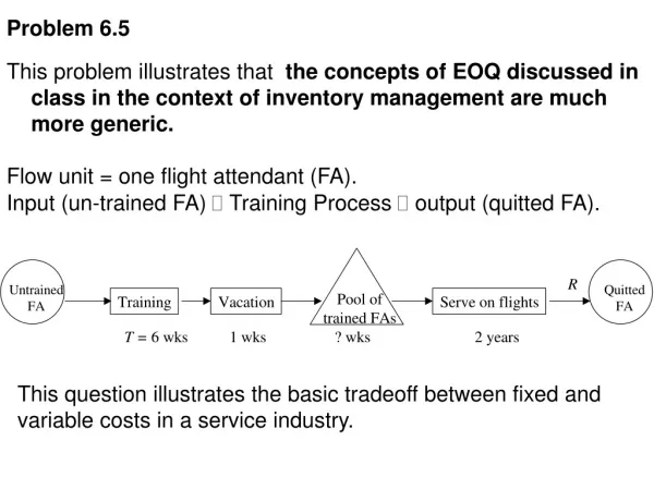
Problem 6.5. This problem illustrates that the concepts of EOQ discussed in class in the context of inventory management are much more generic. Flow unit = one flight attendant (FA). Input (un-trained FA) Training Process output (quitted FA).

Problem 6.5
E N D
Presentation Transcript
Problem 6.5 This problem illustrates that the concepts of EOQ discussed in class in the context of inventory management are much more generic. Flow unit = one flight attendant (FA). Input (un-trained FA) Training Process output (quitted FA). This question illustrates the basic tradeoff between fixed and variable costs in a service industry.
The question asks for the tradeoff between Training costs (higher class size is preferred) versus Holding costs in the buffer (smaller class size) The airline requires a staff of about 1000 I = 1000 Average job tenure being about 2 years T = 2 yrs I = RT R = 500 /yr From inventory model point of view, our product is a trained FA. Inventory carrying cost of a TFA is 500/month H = 6000 /unit/yr
View I Lead time to get the product is 7 weeks Purchasing cost is 6+1 weeks pay (6000/50)7 C = 840 Ordering cost = 10(220+80)6 = 18000 S =18000 EOQ = = 54.77 == 55 units. # of classes = R/Q = 500/55 = 9.091 Cycle inventory = 55/2 = 27.5 The annual cost will be S(R/Q) + H(Q/2) + RC 18000(9.091)+6000(27.5)+500(840) 163636 +165000 + 420000 = 748,636 Inventory cycle = 50/9.091 = 5.5 weeks. 6 weeks to produce. 5.5 weeks to consume
View II Training and vacation is ordering cost Therefore, ordering cost has two parts; Fixed and Variable Fixed Ordering cost = 10(220+80)6 = 18000 Sf =18000 Variable ordering cost is 6+1 weeks pay (6000/50)7 Sv = 840 S = Sf+SvQ His annual cost will be S(R/Q) + H(Q/2) (Sf+SvQ)(R/Q) + H(Q/2) Sf(R/Q) + SvR + H(Q/2) S(R/Q) + CR +H(Q/2) = 748,636 Inventory cycle = 50/9.091 = 5.5 weeks. 6 weeks to produce. 5.5 weeks to consume
(b) Often, in reality, people wish to adopt policies that are simple (e.g., starting training every 6 weeks is simpler than trying to track the exact days to start training when subsequent trainings start every 5.5 weeks. More importantly, for a short period of time (half a week, we need two teams, each with 10 instructor, plus 10 support staff. But what is the implication of deviation from the optimal? Quite small. This is because the optimal cost structure near the (optimal) EOQ is quite flat. If time between classes (T = Q/R ) has to be 6 weeks, Q = T R = (6 wks)×(10 attendants/wk) = 60 attendants. Total Cost of this policy = ($18,000)(500/60) + ($840)(500) + (60/2)($6000) = $750,000 per year. (0.18% increase.) In general, if inventory cycle is less than class cycle (but not too much) we may prefer to set IC = CC to avoid more than one team of instructor/support staff.
View 0 Do not consider EOQ as inventory for 6+1 weeks of training and vacation. It is not easy to solve it then What is the average inventory? It is not EOQ/2 anymore