CASE STUDY Volcker’s Monetary Tightening
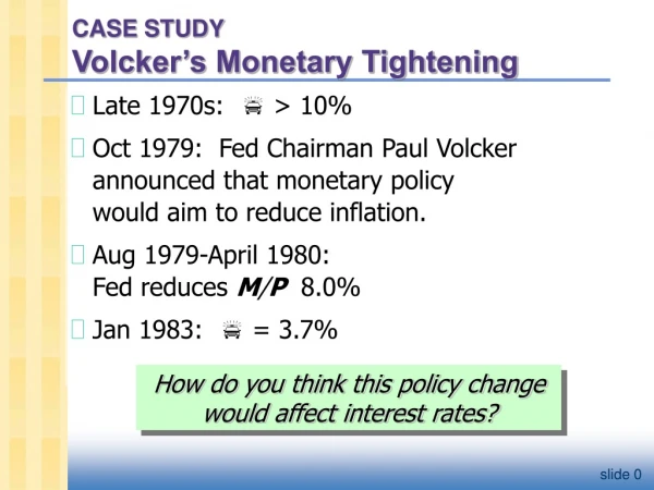
CASE STUDY Volcker’s Monetary Tightening. Late 1970s: > 10% Oct 1979: Fed Chairman Paul Volcker announced that monetary policy would aim to reduce inflation. Aug 1979-April 1980: Fed reduces M / P 8.0% Jan 1983: = 3.7%.

CASE STUDY Volcker’s Monetary Tightening
E N D
Presentation Transcript
CASE STUDY Volcker’s Monetary Tightening • Late 1970s: > 10% • Oct 1979: Fed Chairman Paul Volcker announced that monetary policy would aim to reduce inflation. • Aug 1979-April 1980: Fed reduces M/P 8.0% • Jan 1983: = 3.7% How do you think this policy change would affect interest rates?
The effects of a monetary tightening on nominal interest rates short run long run model prices prediction actual outcome Volcker’s Monetary Tightening, cont. Liquidity Preference (Keynesian) Quantity Theory, Fisher Effect (Classical) sticky flexible i > 0 i < 0 8/1979: i= 10.4% 4/1980: i= 15.8% 1/1983: i= 8.2%
EXERCISE:Analyze shocks with the IS-LM model Use the IS-LM model to analyze the effects of • A boom in the stock market makes consumers wealthier. • After a wave of credit card fraud, consumers use cash more frequently in transactions. For each shock, • use the IS-LM diagram to show the effects of the shock on Y and r. • determine what happens to C, I, and the unemployment rate.
What is the Fed’s policy instrument? What the newspaper says:“the Fed lowered interest rates by one-half point today” What actually happened:The Fed conducted expansionary monetary policy to shift the LM curve to the right until the interest rate fell 0.5 points. The Fed targets the Federal Funds rate: it announces a target value, and uses monetary policy to shift the LM curve as needed to attain its target rate.
What is the Fed’s policy instrument? Why does the Fed target interest rates instead of the money supply? 1) They are easier to measure than the money supply 2) The Fed might believe that LMshocks are more prevalent than ISshocks. If so, then targeting the interest rate stabilizes income better than targeting the money supply.
Interaction between monetary & fiscal policy • Model: monetary & fiscal policy variables (M, G and T ) are exogenous • Real world: Monetary policymakers may adjust Min response to changes in fiscal policy, or vice versa. • Such interaction may alter the impact of the original policy change.
The Fed’s response to G > 0 • Suppose Congress increases G. • Possible Fed responses: 1. hold M constant 2. hold r constant 3. hold Y constant • In each case, the effects of the Gare different:
LM1 r r2 r1 IS2 IS1 Y1 Y2 Y Response 1: hold M constant If Congress raises G, the IScurve shifts right If Fed holds M constant, then LM curve doesn’t shift. Results:
LM1 r LM2 IS2 IS1 Y3 Y1 Y2 Y Response 2: hold r constant If Congress raises G, the IScurve shifts right To keep r constant, Fed increases M to shift LMcurve right. r2 r1 Results:
LM2 LM1 r r3 r1 IS2 IS1 Y1 Y2 Y Response 3: hold Y constant If Congress raises G, the IScurve shifts right To keep Y constant, Fed reduces M to shift LMcurve left. r2 Results:
CASE STUDYThe U.S. economic slowdown of 2001 ~What happened~ 1. Real GDP growth rate 1994-2000: 3.9% (average annual) 2001: 1.2% 2. Unemployment rate Dec 2000: 4.0% Dec 2001: 5.8%
CASE STUDYThe U.S. economic slowdown of 2001 ~Shocks that contributed to the slowdown~ 1. Falling stock prices From Aug 2000 to Aug 2001: -25% Week after 9/11: -12% 2. The terrorist attacks on 9/11 • increased uncertainty • fall in consumer & business confidence Both shocks reduced spending and shifted the IS curve left.
Unemployment (right scale) Real GNP(left scale) The Great Depression
The Spending Hypothesis: Shocks to the IS Curve • asserts that the Depression was largely due to an exogenous fall in the demand for goods & services -- a leftward shift of the IScurve • evidence: output and interest rates both fell, which is what a leftward ISshift would cause
The Spending Hypothesis: Reasons for the IS shift • Stock market crash exogenous C • Oct-Dec 1929: S&P 500 fell 17% • Oct 1929-Dec 1933: S&P 500 fell 71% • Drop in investment • “correction” after overbuilding in the 1920s • widespread bank failures made it harder to obtain financing for investment • Contractionary fiscal policy • in the face of falling tax revenues and increasing deficits, politicians raised tax rates and cut spending
The Money Hypothesis: A Shock to the LM Curve • asserts that the Depression was largely due to huge fall in the money supply • evidence: M1 fell 25% during 1929-33. But, two problems with this hypothesis: • P fell even more, so M/Pactually rose slightly during 1929-31. • nominal interest rates fell, which is the opposite of what would result from a leftward LMshift.
The Money Hypothesis Again: The Effects of Falling Prices • asserts that the severity of the Depression was due to a huge deflation: P fell 25% during 1929-33. • This deflation was probably caused by the fall in M, so perhaps money played an important role after all. • In what ways does a deflation affect the economy?
The Money Hypothesis Again: The Effects of Falling Prices The stabilizing effects of deflation: • P (M/P ) LMshifts right Y • Pigou effect: P (M/P ) consumers’ wealth C IS shifts right Y
The Money Hypothesis Again: The Effects of Falling Prices The destabilizing effects of unexpected deflation:debt-deflation theory P (if unexpected) transfers purchasing power from borrowers to lenders borrowers spend less, lenders spend more if borrowers’ propensity to spend is larger than lenders, then aggregate spending falls, the IScurve shifts left, and Yfalls
The Money Hypothesis Again: The Effects of Falling Prices The destabilizing effects of expected deflation: e r for each value of i I because I = I (r) planned expenditure & agg. demand income & output
Why another Depression is unlikely • Policymakers (or their advisors) now know much more about macroeconomics: • The Fed knows better than to let M fall so much, especially during a contraction. • Fiscal policymakers know better than to raise taxes or cut spending during a contraction. • Federal deposit insurance makes widespread bank failures very unlikely. • Automatic stabilizers make fiscal policy expansionary during an economic downturn.

