Thermodynamics
Thermodynamics. Begin with a brief review of Chapter 5. Natural systems tend toward states of minimum energy. Energy States. Unstable: falling or rolling. Stable: at rest in lowest energy state. Metastable: in low-energy perch.

Thermodynamics
E N D
Presentation Transcript
Thermodynamics • Begin with a brief review of Chapter 5 Natural systems tend toward states of minimum energy
Energy States • Unstable: falling or rolling • Stable: at rest in lowest energy state • Metastable: in low-energy perch Figure 5-1. Stability states. Winter (2001) An Introduction to Igneous and Metamorphic Petrology. Prentice Hall.
Gibbs Free Energy Gibbs free energy is a measure of chemical energy Gibbs free energy for a phase: G = H - TS Where: G = Gibbs Free Energy H = Enthalpy (heat content) T = Temperature in Kelvins S = Entropy (can think of as randomness)
Thermodynamics DG for a reaction of the type: 2 A + 3 B = C + 4 D DG = S (n G)products - S(n G)reactants = GC + 4GD - 2GA - 3GB The side of the reaction with lower G will be more stable
z z P T 2 2 - = - G G VdP SdT T P T P 2 2 1 1 P T 1 1 Thermodynamics For other temperatures and pressures we can use the equation: dG = VdP - SdT (ignoring DX for now) where V = volume and S = entropy (both molar) We can use this equation to calculate G for any phase at any T and P by integrating If V and S are constants, our equation reduces to: GT2 P2 - GT1 P1 = V(P2 - P1) - S (T2 - T1)
Now consider a reaction, we can then use the equation: dDG = DVdP - DSdT (again ignoring DX) DG for any reaction = 0 at equilibrium
Worked Problem #2 used: dDG = DVdP - DSdT and G, S, V values for albite, jadeite and quartz to calculate the conditions for which DG of the reaction: Ab + Jd = Q is equal to 0 Method: • from G values for each phase at 298K and 0.1 MPa calculate DG298, 0.1 for the reaction, do the same for DV and DS • DG at equilibrium = 0, so we can calculate an isobaric change in T that would be required to bring DG298, 0.1 to 0 0 - DG298, 0.1 = -DS (Teq - 298) (at constant P) • Similarly we could calculate an isothermal change 0 - DG298, 0.1 = -DV (Peq - 0.1) (at constant T)
NaAlSi3O8 = NaAlSi2O6 + SiO2 P - T phase diagram of the equilibrium curve How do you know which side has which phases? Figure 27-1. Temperature-pressure phase diagram for the reaction: Albite = Jadeite + Quartz calculated using the program TWQ of Berman (1988, 1990, 1991). Winter (2001) An Introduction to Igneous and Metamorphic Petrology. Prentice Hall.
D dP S = Thus D dT V pick any two points on the equilibrium curve dDG = 0 = DVdP - DSdT Figure 27-1. Temperature-pressure phase diagram for the reaction: Albite = Jadeite + Quartz calculated using the program TWQ of Berman (1988, 1990, 1991). Winter (2001) An Introduction to Igneous and Metamorphic Petrology. Prentice Hall.
z P 2 - = G G VdP P P 2 1 P 1 Gas Phases Return to dG = VdP - SdT, for an isothermal process: For solids it was fine to ignore V as f(P) For gases this assumption is shitty You can imagine how a gas compresses as P increases How can we define the relationship between V and P for a gas?
Gas Pressure-Volume Relationships Ideal Gas • As P increases V decreases • PV=nRTIdeal Gas Law • P = pressure • V = volume • T = temperature • n = # of moles of gas • R = gas constant = 8.3144 J mol-1 K-1 Figure 5-5. Piston-and-cylinder apparatus to compress a gas. Winter (2001) An Introduction to Igneous and Metamorphic Petrology. Prentice Hall. P x V is a constant at constant T
z P 2 - = G G VdP P P 2 1 P 1 z RT P 2 - = G G dP P P P 2 1 P 1 1 P 2 - = G G RT dP P P P 2 1 P 1 Gas Pressure-Volume Relationships Since we can substitute RT/P vor V (for a single mole of gas), thus: and, since R and T are certainly independent of P: z
z 1 = dx ln x x Gas Pressure-Volume Relationships And since GP2 - GP1 = RT ln P2 - ln P1 = RT ln (P2/P1) Thus the free energy of a gas phase at a specific P and T, when referenced to a standard atate of 0.1 MPa becomes: GP, T - GT = RT ln (P/Po) G of a gas at some P and T = G in the reference state (same T and 0.1 MPa) + a pressure term o
Gas Pressure-Volume Relationships The form of this equuation is very useful GP, T - GT = RT ln (P/Po) For a non-ideal gas (more geologically appropriate) the same form is used, but we substitute fugacity ( f ) for P wheref = gPg is the fugacity coefficient Tables of fugacity coefficients for common gases are available At low pressures most gases are ideal, but at high P they are not o
Dehydration Reactions • Mu + Q = Kspar + Sillimanite + H2O • We can treat the solids and gases separately GP, T - GT = DVsolids (P - 0.1) + RT ln (P/0.1) (isothermal) • The treatment is then quite similar to solid-solid reactions, but you have to solve for the equilibrium P by iteration
D dP S = D dT V Dehydration Reactions(qualitative analysis) Figure 27-2. Pressure-temperature phase diagram for the reaction muscovite + quartz = Al2SiO5 + K-feldspar + H2O, calculated using SUPCRT (Helgeson et al., 1978). Winter (2001) An Introduction to Igneous and Metamorphic Petrology. Prentice Hall.
Solutions: T-X relationships Ab = Jd + Q was calculated for pure phases When solid solution results in impure phases the activity of each phase is reduced Use the same form as for gases (RT ln P or ln f) Instead of fugacity, we use activity Ideal solution: ai = Xi n = # of sites in the phase on which solution takes place Non-ideal: ai = gi Xi where gi is the activity coefficient n n
Solutions: T-X relationships Example: orthopyroxenes (Fe, Mg)SiO3 • Real vs. Ideal Solution Models Figure 27-3. Activity-composition relationships for the enstatite-ferrosilite mixture in orthopyroxene at 600oC and 800oC. Circles are data from Saxena and Ghose (1971); curves are model for sites as simple mixtures (from Saxena, 1973) Thermodynamics of Rock-Forming Crystalline Solutions. Winter (2001) An Introduction to Igneous and Metamorphic Petrology. Prentice Hall.
D = D - o c d G G RT K a a ln = c D K P , T P , T a b a a A B Solutions: T-X relationships Back to our reaction: Simplify for now by ignoring dP and dT For a reaction such as: aA + bB = cC + dD At a constant P and T: where:
Pyx Q X X = Jd SiO 2 K Plag X Ab Compositional variations Effect of adding Ca to albite = jadeite + quartz plagioclase = Al-rich Cpx + Q DGT, P = DGoT, P + RTlnK Let’s say DGoT, Pwas the value that we calculated for equilibrium in the pure Na-system (= 0 at some P and T) DGoT, P = DG298, 0.1 + DV (P - 0.1) - DS (T-298) = 0 By adding Ca we will shift the equilibrium by RTlnK We could assume ideal solution and All coefficients = 1
Pyx X Jd Plag X Ab Compositional variations So now we have: DGT, P = DGoT, P + RTlnsince Q is pure DGoT, P = 0 as calculated for the pure system at P and T DGT, P is the shifed DG due to the Ca added (no longer 0) Thus we could calculate a DV(P-Peq) that would bring DGT, P back to 0, solving for the new Peq
Compositional variations Effect of adding Ca to albite = jadeite + quartz DGP, T = DGoP, T + RTlnK numbers are values for K Figure 27-4. P-T phase diagram for the reaction Jadeite + Quartz = Albite for various values of K. The equilibrium curve for K = 1.0 is the reaction for pure end-member minerals (Figure 27-1). Data from SUPCRT (Helgeson et al., 1978). Winter (2001) An Introduction to Igneous and Metamorphic Petrology. Prentice Hall.
Geothermobarometry Use measured distribution of elements in coexisting phases from experiments at known P and T to estimate P and T of equilibrium in natural samples
Geothermobarometry The Garnet - Biotite geothermometer
Geothermobarometry The Garnet - Biotite geothermometer lnKD = -2108 · T(K) + 0.781 DGP,T = 0 = DH 0.1, 298 - TDS0.1, 298 + PDV + 3 RTlnKD Figure 27-5. Graph of lnK vs. 1/T (in Kelvins) for the Ferry and Spear (1978) garnet-biotite exchange equilibrium at 0.2 GPa from Table 27-2. Winter (2001) An Introduction to Igneous and Metamorphic Petrology. Prentice Hall.
Geothermobarometry The Garnet - Biotite geothermometer Figure 27-6. AFM projections showing the relative distribution of Fe and Mg in garnet vs. biotite at approximately 500oC (a) and 800oC (b). From Spear (1993) Metamorphic Phase Equilibria and Pressure-Temperature-Time Paths. Mineral. Soc. Amer. Monograph 1.
Geothermobarometry The Garnet - Biotite geothermometer Figure 27-7. Pressure-temperature diagram similar to Figure 27-4 showing lines of constant KD plotted using equation (27-35) for the garnet-biotite exchange reaction. The Al2SiO5 phase diagram is added. From Spear (1993) Metamorphic Phase Equilibria and Pressure-Temperature-Time Paths. Mineral. Soc. Amer. Monograph 1.
Geothermobarometry The GASP geobarometer Figure 27-8. P-T phase diagram showing the experimental results of Koziol and Newton (1988), and the equilibrium curve for reaction (27-37). Open triangles indicate runs in which An grew, closed triangles indicate runs in which Grs + Ky + Qtz grew, and half-filled triangles indicate no significant reaction. The univariant equilibrium curve is a best-fit regression of the data brackets. The line at 650oC is Koziol and Newton’s estimate of the reaction location based on reactions involving zoisite. The shaded area is the uncertainty envelope. After Koziol and Newton (1988) Amer. Mineral., 73, 216-233
Geothermobarometry The GASP geobarometer Figure 27-8. P-T diagram contoured for equilibrium curves of various values of K for the GASP geobarometer reaction: 3 An = Grs + 2 Ky + Qtz. From Spear (1993) Metamorphic Phase Equilibria and Pressure-Temperature-Time Paths. Mineral. Soc. Amer. Monograph 1.
Geothermobarometry Figure 27-10. P-T diagram showing the results of garnet-biotite geothermometry (steep lines) and GASP barometry (shallow lines) for sample 90A of Mt. Moosilauke (Table 27-4). Each curve represents a different calibration, calculated using the program THERMOBAROMETRY, by Spear and Kohn (1999). The shaded area represents the bracketed estimate of the P-T conditions for the sample. The Al2SiO5 invariant point also lies within the shaded area.
Geothermobarometry Figure 27-11. P-T phase diagram calculated by TQW 2.02 (Berman, 1988, 1990, 1991) showing the internally consistent reactions between garnet, muscovite, biotite, Al2SiO5 and plagioclase, when applied to the mineral compositions for sample 90A, Mt. Moosilauke, NH. The garnet-biotite curve of Hodges and Spear (1982) Amer. Mineral., 67, 1118-1134 has been added.
Geothermobarometry P-T-t Paths Figure 27-12. Chemically zoned plagioclase and poikiloblastic garnet from meta-pelitic sample 3, Wopmay Orogen, Canada. a. Chemical profiles across a garnet (rim rim). b. An-content of plagioclase inclusions in garnet and corresponding zonation in neighboring plagioclase. After St-Onge (1987) J. Petrol. 28, 1-22 .
Geothermobarometry P-T-t Paths Figure 27-13. The results of applying the garnet-biotite geothermometer of Hodges and Spear (1982) and the GASP geobarometer of Koziol (1988, in Spear 1993) to the core, interior, and rim composition data of St-Onge (1987). The three intersection points yield P-T estimates which define a P-T-t path for the growing minerals showing near-isothermal decompression. After Spear (1993).
Geothermobarometry Precision and Accuracy Figure 27-14. An illustration of precision vs. accuracy. a. The shots are precise because successive shots hit near the same place (reproducibility). Yet they are not accurate, because they do not hit the bulls-eye. b. The shots are not precise, because of the large scatter, but they are accurate, because the average of the shots is near the bulls-eye. c. The shots are both precise and accurate. Winter (2001) An Introduction to Igneous and Metamorphic Petrology. Prentice Hall.
Geothermobarometry Precision and Accuracy Figure 27-15. P-T diagram illustrating the calculated uncertainties from various sources in the application of the garnet-biotite geothermometer and the GASP geobarometer to a pelitic schist from southern Chile. After Kohn and Spear (1991b) Amer. Mineral., 74, 77-84 and Spear (1993) From Spear (1993) Metamorphic Phase Equilibria and Pressure-Temperature-Time Paths. Mineral. Soc. Amer. Monograph 1.
Figure 27-16. Phase diagram for the reaction: calcite + quartz = wollastonite + CO2 calculated using the program SUPCRT, assuming pCO2 = PLith. Winter (2001) An Introduction to Igneous and Metamorphic Petrology. Prentice Hall.