14 Vector Autoregressions, Unit Roots, and Cointegration
420 likes | 1.42k Vues
14 Vector Autoregressions, Unit Roots, and Cointegration. What is in this Chapter?. This chapter discusses work on time-series analysis starting in the 1980s. First there is a discussion of vector autoregression models, Next we talk of the different unit root tests.

14 Vector Autoregressions, Unit Roots, and Cointegration
E N D
Presentation Transcript
What is in this Chapter? • This chapter discusses work on time-series analysis starting in the 1980s. • First there is a discussion of vector autoregression models, • Next we talk of the different unit root tests. • Finally, we discuss cointegration, which is a method of analyzing long-run relationships between nonstationary variables. We discuss tests for cointegration and estimation of cointegrating relationships
14.2 Vector Autoregressions • In previous sections we discussed the analysis of a single time series • When we have several time series, we need to take into account the interdependence between them • One way of doing this is to estimate a simultaneous equations model as discussed in Chapter 9 but with lags in all the variables • Such a model is called a dynamic simultaneous equations model
14.2 Vector Autoregressions • However, this formulation involves two steps: • first, we have to classify the variables into two categories, endogenous and exogenous, • second, we have toimpose some constraints on the parameters to achieve identification. • Sims argues that both these steps involve many arbitrary decisions and suggests as an alternative, the vectorautoregression (VAR) approach. • This is just a multiple time-series generalization of the AR model. • The VAR model is easy to estimate because we can use the OLS method
14.3 Problems with VAR Models in Practice • We have considered only a simple model with two variables and only one lag for each. • In practice, since we are not considering any moving average errors, the autoregressions would probably have to have more lags to be useful for prediction • Otherwise, univariate ARMA models would do better.
14.3 Problems with VAR Models in Practice • Suppose that we consider say six lags for each variable and we have a small system with four variables • Then each equation would have 24 parameters to be estimated and we thus have 96 parameters to estimate overall • This overparameterization is one of the major problems with VAR models.
14.3 Problems with VAR Models in Practice • One such model that has been found particularly useful in prediction is the Bayesian vectorautoregression (BVAR) • In BVAR we assign some prior distributions for the coefficients in the vector autoregressions • In each equation, the coefficient of the own lagged variable has a prior mean 1, all others have prior means 0, with the variance of the prior decreasing as the lag length increases • For instance, with two variables y1t and y2t and four lags for each, the first equation will be
14.5 Unit Root Tests • The Low Power of Unit Root Tests • Schwert (1989) first presented Monte Carlo evidence to point out the size distortion problems of the commonly used unit root tests: the ADF and PP tests. • Whereas Schwert complained about size distortions, DeJong et al. complained about the low power of unit root tests • They argued that the unit root tests have low power against plausible trend-stationary alternatives
14.5 Unit Root Tests • They argue that the PP tests have very low power (generally less than 0.10) against trend-stationary alternatives but the ADF test has power approaching 0.33 and thus is likely to be more useful in practice. • They conclude that tests with higher power need to be developed
14.5 Unit Root Tests • Structural Change and Unit Roots • In all the studies on unit roots, the issue of whether a time series is of the DS or TS type was decided by analyzing the series for the entire time period during which many major events took place • The Nelson-Plosser series, for instance, covered the period 1909-1970,which includes the two world wars and the Depression of the 1930s
14.5 Unit Root Tests • If there have been any changes in the trend because of these events, the results obtained by assuming a constant parameter structure during the entire period will be suspect • Many studies done using the traditional multiple regression methods have included dummy variables (see Sections 8.2 and 8.3) to allow for different intercepts (and slopes) • Rappoport and Richlin (1989) show that a segmented trend model is a feasible alternative to the DS model.
14.5 Unit Root Tests • Perron (1989) argues that standard tests for the unit root hypothesis against the trend-stationary (TS) alternatives cannot reject the unit root hypothesis if the time series has a structural break. • Of course, one can also construct examples where, for instance • y1, y2, • • •, ym is a random walk with drift • ym+1, ..., ym+n is another random walk with a different drift • and the combined series is not the DS type
14.5 Unit Root Tests • Perron's study was criticized on the argument that he "peeked at the data" before analysis—that after looking at the graph, he decided that there was a break • But Kim (1990), using Bayesian methods, finds that even allowing for an unknown breakpoint, the standard tests of the unit root hypothesis were biased in favor of accepting the unit root hypothesis if the series had a structural break at some intermediate date.
14.5 Unit Root Tests • When using long time series, as many of these studies have done, it is important to take account of structural changes. Parameter constancy tests have frequently been used in traditional regression analysis.
14.6 Cointegration • In the Box-Jenkins method, if the time series is nonstationary (as evidenced by the correlogram not damping), we difference the series to achieve stationarity and then use elaborate ARMA models to fit the stationary series. • When we are considering two time series, yt and Xt say, we do the same thing. • This differencing operation eliminates the trend or long-term movement in the series
14.6 Cointegration • However, what we may be interested in is explaining the relationship between the trends in yt and Xt • We can do this by running a regression of Yt on Xt, but this regression will not make sense if a long-run relationship does not exist. • By asking the question of whether yt and Xt are cointegrated, we are asking whether there is any long-run relationship between the trends in yt and xt.
14.6 Cointegration • The case with seasonal adjustment is similar • Instead of eliminating the seasonal components from y and x and then analyzing the de-seasonalized data, we might also be asking whether there is a relationship between the seasonals in y and x • This is the idea behind "seasonal cointegration. • Note that in this case we do not considerfirst differences or I(1) processes • For instance, with monthly data we consider twelfthdifferences yt-yt-12 Similarly, for Xt we consider Xt-Xt-12
14.9 Cointegration and Error Correction Models • If xt and yt are cointegrated, there is a long-run relationship between them • Furthermore, the short-run dynamics can be described by the error correction model (ECM) • This is known as the Granger representation theorem • If Xt ~ I(1), yt ~I(1), and zt = yt -βxt is I(0), then x and y are said to be cointegrated • The Granger representation theorem says that in this case Xt and yt may be considered to be generated by ECMs: