A grid implementation of a GRASP-ILS heuristic for the mirrored traveling tournament problem
A grid implementation of a GRASP-ILS heuristic for the mirrored traveling tournament problem Aletéia ARAÚJO Vinod REBELLO Celso RIBEIRO Sebastián URRUTIA Summary Motivation The Mirrored Traveling Tournament Problem Extended GRASP + ILS heuristic Construction phase Neighborhoods

A grid implementation of a GRASP-ILS heuristic for the mirrored traveling tournament problem
E N D
Presentation Transcript
A grid implementation of a GRASP-ILS heuristic for the mirrored traveling tournament problem Aletéia ARAÚJO Vinod REBELLO Celso RIBEIRO Sebastián URRUTIA
Summary • Motivation • The Mirrored Traveling Tournament Problem • Extended GRASP + ILS heuristic • Construction phase • Neighborhoods • Parallel implementations of GRASP-ILS • PAR-MP • Computational results • EsporteMax: optimization in sports management and scheduling
Motivation • Game scheduling is a difficult task, involving different types of constraints, logistic issues, multiple objectives, and several decision makers. • Total distance traveled is an important variable to be minimized, to reduce traveling costs and to give more time to the players for resting and training. • Timetabling is the major area of applications of OR in sports.
Formulation • Traveling Tournament Problem (TTP) • n (even) teams take part in a tournament. • Each team has its own stadium at its home city. • Distances between the stadiums are known. • A team playing two consecutive away games goes directly from one city to the other, without returning to its home city.
Formulation • Tournament is a strict double round-robin tournament: • There are 2(n-1) rounds, each one with n/2 games. • Each team plays against every other team twice, one at home and the other away. • No team can play more than three games in a home stand (home games) or in a road trip (away games). • Goal: minimize the total distance traveled by all teams.
Formulation Mirrored Traveling Tournament Problem (MTTP): All teams face each other once in the first phase with n-1 rounds. In the second phase with the last n-1 rounds, the teams play each other again in the same order, following an inverted home/away pattern. Common structure in Latin-American tournaments. Set of feasible solutions for the MTTP is a subset of the feasible solutions for the TTP.
1-Factorizations • Given a graph G=(V, E), a factor of G is a graph G’=(V,E’) with E’E. • G’ is a 1-factor if all its nodes have degree equal to one. • A factorization of G=(V,E) is a set of edge-disjoint factors G1=(V,E1), ..., Gp=(V,Ep), such that E1...Ep=E. • All factors in a 1-factorization of G are 1-factors. • Oriented 1-factorization: assign orientations to the edges of a 1-factorization
1-Factorizations 1 2 5 4 3 6 • Mirrored tournament: games in the second phase are determined by those in the first. • Each edge of Kn represents a game. • Each 1-factor of Kn represents a round. • Each ordered oriented 1-factorization of Kn represents a feasible schedule for n teams. • Example: K6
1-Factorizations 1 1 1 1 1 2 2 2 2 2 5 5 5 5 5 4 4 4 4 4 3 3 3 3 3 6 6 6 6 6
Constructive heuristic • Three steps: • Schedule games using abstract teams: polygon method defines the structure of the tournament • Assign real teams to abstract teams: greedy heuristic to QAP (number of travels between stadiums of the abstract teams x distances between the stadiums of the real teams) • Select stadium for each game (home/away pattern) in the first phase (mirrored tournament): • Build a feasible assignment of stadiums, starting from a random assignment of stadiums in the first round. • Improve this assignment of stadiums, using a simple local search algorithm based on home-away swaps.
Constructive heuristic 6 Example: “polygon method” for n=6 1 5 2 1st round 3 4
Constructive heuristic 6 Example: “polygon method” for n=6 5 4 1 2nd round 2 3
Constructive heuristic 6 Example: “polygon method” for n=6 4 3 5 3rd round 1 2
Constructive heuristic 6 Example: “polygon method” for n=6 3 2 4 4th round 5 1
Constructive heuristic 6 Example: “polygon method” for n=6 2 1 3 5th round 4 5
Constructive heuristic • Step 2: assign real teams to abstract teams • Build a matrix with the number of consecutive games for each pair of abstract teams: • For each pair of teams X and Y, an entry in this matrix contains the total number of times in which the other teams play consecutively with X and Y in any order. • Greedily assign pairs of real teams with close home cities to pairs of abstract teams with large entries in the matrix with the number of consecutive games: QAP heuristic
Constructive heuristic • Step 3: select stadium for each game in the first phase of the tournament: • Two-part strategy: • Build a feasible assignment of stadiums, starting from a random assignment in the first round. • Improve the assignment of stadiums, performing a simple local search algorithm based on home-away swaps.
Neighborhood home-away swap (HAS) 1 1 1 1 1 2 2 2 2 2 5 5 5 5 5 4 4 4 4 4 3 3 3 3 3 6 6 6 6 6
Neighborhood home-away swap (HAS) 1 1 1 1 2 2 2 2 5 5 5 5 4 4 4 4 3 3 3 3 6 6 6 6 1 2 5 4 3 6
Neighborhood team-swap (TS) 1 1 1 1 1 2 2 2 2 2 5 5 5 5 5 4 4 4 4 4 3 3 3 3 3 6 6 6 6 6
Neighborhood team-swap (TS) 2 2 2 2 2 1 1 1 1 1 5 5 5 5 5 4 4 4 4 4 3 3 3 3 3 6 6 6 6 6
Neighborhood partial round swap (PRS) 1 2 1 2 3 8 3 8 7 4 7 4 6 5 6 5
Neighborhood partial round swap (PRS) 1 2 1 2 3 8 3 8 7 4 7 4 6 5 6 5
Ejection chain: game rotation (GR) • Neigborhood “game rotation” (GR) (ejection chain): • Enforce a game to be played at some round: add a new edge to a 1-factor of the 1-factorization associated with the current schedule. • Use an ejection chain to recover a 1-factorization.
Ejection chain: game rotation (GR) 1 1 1 1 1 2 2 2 2 2 5 5 5 5 5 4 4 4 4 4 3 3 3 3 3 6 6 6 6 6
Ejection chain: game rotation (GR) 1 1 1 2 5 2 2 5 5 4 4 3 3 4 3 6 6 6 1 1 2 5 2 5 4 3 4 3 6 6 Enforce game (1,3) to be played in round 2
Ejection chain: game rotation (GR) 1 1 1 2 5 2 2 5 5 4 4 3 3 4 3 6 6 6 1 1 2 5 2 5 4 3 4 3 6 6 Enforce game (1,3) to be played in round 2
Ejection chain: game rotation (GR) 1 1 1 2 5 2 2 5 5 4 4 3 3 4 3 6 6 6 1 1 2 5 2 5 4 3 4 3 6 6
Ejection chain: game rotation (GR) 1 1 1 2 5 2 2 5 5 4 4 3 3 4 3 6 6 6 1 1 2 5 2 5 4 3 4 3 6 6
Ejection chain: game rotation (GR) 1 1 1 2 5 2 2 5 5 4 4 3 3 4 3 6 6 6 1 1 2 5 2 5 4 3 4 3 6 6
Ejection chain: game rotation (GR) 1 1 1 2 5 2 2 5 5 4 4 3 3 4 3 6 6 6 1 1 2 5 2 5 4 3 4 3 6 6
Ejection chain: game rotation (GR) 1 1 1 2 5 2 2 5 5 4 4 3 3 4 3 6 6 6 1 1 2 5 2 5 4 3 4 3 6 6
Ejection chain: game rotation (GR) 1 1 1 2 5 2 2 5 5 4 4 3 3 4 3 6 6 6 1 1 2 5 2 5 4 3 4 3 6 6
Ejection chain: game rotation (GR) 1 1 1 2 5 2 2 5 5 4 4 3 3 4 3 6 6 6 1 1 2 5 2 5 4 3 4 3 6 6 Ejection chain moves are able to find solutions unreachable with other neighborhoods.
Neighborhoods • Only movements in neighborhoods PRS and GR may change the structure of the initial schedule. • However, PRS moves not always exist, due to the structure of the solutions built by polygon method e.g. for n = 6, 8, 12, 14, 16, 20, 24. • PRS moves may appear after an ejection chain move is made. • The ejection chain move is able to find solutions that are not reachable through other neighborhoods: escape from local optima
GRASP + ILS heuristic • Hybrid improvement heuristic for the MTTP: • Combination of GRASP and ILS metaheuristics. • Initial solutions: randomized version of the constructive heuristic. • Local search with first improving move: use TS, HAS, PRS, and HAS cyclically in this order until a local optimum for all neighborhoods is found. • Perturbation: random movement in GR neighborhood. • Detailed algorithm to appear in EJOR.
GRASP + ILS heuristic while .not.StoppingCriterion S BuildGreedyRandomizedSolution() S, S LocalSearch(S) repeat S’ Perturbation(S) S’ LocalSearch(S’) S AceptanceCriterion(S,S’) S* UpdateGlobalBestSolution(S,S*) S UpdateIterationBestSolution(S,S) until ReinitializationCriterion end GRASP construction phase ILS phase
Parallel implementations of metaheuristics • Robustness • Granularity: coarse grain implementation suitable to grid environments (communication) • Master-slave • Single-walk vs. multiple-walk • Cooperative vs. independent • Cost and frequency of communication: few communication steps • Nature of the information to be shared
Parallel strategy PAR-I • Parallel strategy with independent processes. • PAR-I is equivalent to running the sequential algorithm simultaneously on multiple machines. • After receiving the seed, each process computes a new solution. • Then, each process runs an ILS local search phase until the reinitialization criterion is met. • Procedure stops when a solution at least as good as a given target is found.
Parallel strategy PAR-O • Parallel strategy with one-off cooperation. • Identical to PAR-I, except for the first iteration of the main loop. • After each process executes the first GRASP construction phase, the initial solution found by each of them is sent to the master. • The master selects and broadcats the best initial solution to all procesors.
Parallel strategy PAR-O • All workers run the ILS local search phase of the first iteration using the same initial solution. • The following iterations are executed independently. • Processors stop ILS phase after 50 steps deteriorating solution quality. • This strategy is called one-off cooperation because exchange only occurs at the first iteration.
Parallel strategy PAR-1P • Master manages the exchange of information collected along the trajectories investigated by each worker. • It keeps the best solution found by any worker. • Each time the best solution is improved, the master broadcasts its cost to all workers. • The idea is to use this information not only to converge faster to a target solution, but also to find better solutions than the independent search strategies.
Parallel strategy PAR-1P • Each time a worker completes the ILS phase, it will compare the cost of the solution found with that of the best solution held by the master. • If it is better, the worker sends its solution to the master, otherwise the solution is discarded. • Then, the worker chooses between two possibilities: • It requests the best solution held by the master to start the ILS local search phase with this solution; or • The worker restarts from the GRASP construction phase • Workers indirectly exchange elite solutions found along their search trajectories.
Parallel strategy PAR-MP • Master handles a centralized pool of elite solutions, collecting and distributing them upon request. • Slaves start their searches from different initial solutions. • Slaves exchange and share elite solutions found along their search trajectories. • Master updates the pool of elite solutions with a newly received solution according to some criteria based on the quality and diversity of the solutions already in the pool.
Parallel strategy PAR-MP • When a slave completes an iteration (ILS phase), it can either request an elite solution from the pool or construct a new initial solution randomly. • To guarantee diversity within the pool, the insertion of a new solution depends on the state of the pool and on how this solution was generated. • When a slave requests an elite solution from the master, a solution is selected at random from the pool and sent back to it.
Computational results • Circular instances with n = 12, ..., 20 teams. • MLB instances with n = 12, ..., 16 teams. • All available from http://mat.gsia.cmu.edu/TOURN/ • Largest unmirrored instances exactly solved to date: n=6 (sequential), n=8 (parallel) • Random number generator: Mersenne Twister of Matsumoto and Nishimura. • Algorithms implemented using C++ and MPI-LAM (version 7.0.6).