Download
1 / 16
160 likes | 358 Vues
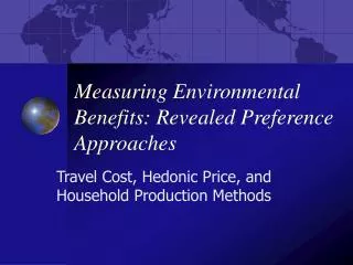
Measuring Environmental Benefits: Revealed Preference Approaches. Travel Cost, Hedonic Price, and Household Production Methods. Revealed preference approaches. Travel Cost Model : use data from actual vistations, estimate cost of travel, derive demand curve for visits to the “site”.

E N D
Measuring Environmental Benefits: Revealed Preference Approaches Travel Cost, Hedonic Price, and Household Production Methods
Revealed preference approaches • Travel Cost Model: use data from actual vistations, estimate cost of travel, derive demand curve for visits to the “site”. • Hedonic Price Method: compare products with similar attributes but one “bundles” an environmental good, derive demand for the environmental good. • Household Production Model: households (people) bundle environmental goods with private goods to produce experience that enhances utility
Travel Cost Model: ANWR • What is the use-value of Arctic National Wildlife Reserve? • Current entrance fee = 0. Is the value = 0? • v = # visits person makes to ANWR, • X = other goods purchased by person, • L = # hours worked by person at wage w. • P0 = out-of-pocket expenses to visit ANWR, • F = entrance fee.
Effective price of trip • t = travel time, s = visit time • Price of a trip: p = [P0+w(t+s) + F] • Notice opportunity cost of time • This assumes we value travel time and visitation time at the wage rate of the individual. • Value of time ranges, but is often estimated at 1/3 or 1/2 the wage rate.
Objective • Want to derive a demand curve for visits to ANWR. • Will allow us to calculate consumer surplus • Can calculate use-value of ANWR • Can determine cost to consumers from e.g. entrance fee (from 0 to F1)
Demand for visits to ANWR $ . NEW Consumer Surplus . . . . . OLD Consumer Surplus . . . . . . F1 . . . Demand . F0 V1 Visits V0
Procedure [1 of 2] • Station students at park entrance on several “random” days. • Ask visitors (1) zip code, (2) others (mode of travel, $ spent, socioeconomic…) • Scale up to entire year, over entire pop: • # visits/zip code/year • Calculate travel cost from each zip code • Divide into “zones” of equal travel cost • E.g. Northern Alaska, Southern Alaska, BC, … lower 48, etc.
Travel cost “zones” Site Z=1 Z=4 Z=3 Z=2 Zones have equal travel cost within each zone.
Procedure [2 of 2] • Calculate population (Pz) and estimated number of visits (Sz) from each “zone”. • Calculate visitation rate: Vz = Sz/Pz. • Plot price (pz+F) vs. visitation rate (Vz). Pricez . . . . . . . . . Vz
Hedonic Price Method: Urban Creeks • Proposal to restore an urban creek. Costs easy to calculate, benefits more difficult. • Benefit of restoring an urban creek? • Basic idea: House prices (or other market goods) reflect quality of attributes. One attribute is proximity to nice creek. • Ceteris paribus, houses near creek should be more valuable
If all houses identical • Suppose all houses are identical in every respect except different distances from nice creek. House Price (P) Use regression to estimate a “hedonic price function” . . . . . . . Dist to creek (d)
Value of a clean creek • Suppose we look at houses at distances 0 miles, 1 mile, 2 miles, etc... • H(d) = # houses at distance d, (H=total #) • Value of the creek is increase in value of housing stock with and without the creek: • [H(0)*P(0) + H(1)*P(1) +… ] – [SH(i)*P()] • Explain formula.
But all houses are not identical • Want to “control” for other characteristics of house that affect its price. • Size (s), age (a), schools (h), condition (c), view (v), etc. • P(d) becomes P(s, a, h, c, v, …) – use multiple regression instead of single. • Rest of analysis is same. • Note: For continuous change (small change in noise from SBA changing flight schedules) calculate “marginal damage from noise”.
Hedonic pricing to value risks • What is the cost of additional occupational risk? • Hedonics provides a way to estimate. • Compare different occupations with different risks of mortality, estimate hedonic price function
Hedonic price function Wage Calculate W(p). dW/dp = marginal value of risk “Value of Statistical Life” is found By extrapolating to p = 1.0. VSL typically $3-$6 million . VSL . . . . . . Prob death (p) … 1.0 .0001 .0002