Chapter 4. Microwave Network Analysis
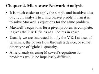
Chapter 4. Microwave Network Analysis. It is much easier to apply the simple and intuitive idea of circuit analysis to a microwave problem than it is to solve Maxwell’s equations for the same problem.

Chapter 4. Microwave Network Analysis
E N D
Presentation Transcript
Chapter 4. Microwave Network Analysis • It is much easier to apply the simple and intuitive idea of circuit analysis to a microwave problem than it is to solve Maxwell’s equations for the same problem. • Maxwell’s equations for a given problem is complete, it gives the E & H fields at all points in space. • Usually we are interested in only the V & I at a set of terminals, the power flow through a device, or some other type of “global” quantity. • A field analysis using Maxwell’s equations for problems would be hopelessly difficult.
4.1 Impedance and Equivalent Voltages and Currents Equivalent Voltages and Currents • The voltage of the + conductor relative to the – conductor • After having defined and determined a voltage, current, and characteristic impedance, we can proceed to apply the circuit theory for transmission lines to characterize this line as a circuit element.
Figure 4.1 (p. 163)Electric and magnetic field lines for an arbitrary two-conductor TEM line.
Figure 4.2 (p. 163)Electric field lines for the TE10 mode of a rectangular waveguide.
There is no “correct” voltage in the sense of being unique. • There are many ways to define equivalent voltage, current, and impedance for waveguides. • V&I are defined only for a particular waveguide mode. • The equivalent V&I should be defined so that their product gives the power flow of the mode. • V/I for a single traveling wave should be equal to Z0 of the line. This impedance may be chosen arbitrarily, but is usually selected as equal to the wave impedance of the line.
For an arbitrarily waveguide mode, the transverse fields where e and h are the transverse field variations of the mode. Since Et & Htare related by Zw, • Defining equivalent voltage and current waves as
The complex power flow for the incident wave • Since we want this power to be (1/2)V+I+*, where the surface integration is over the cross section of the waveguide. • If it is desired to have Z0 = Zw,
For higher order modes, • Ex 4.1
The Concept of Impedance • Various types of impedance • Intrinsic impedance ( ) of the medium: depends on the material parameters of the medium, and is equal to the wave impedance for plane waves. • Wave impedance ( ): a characteristic of the particular type of wave. TEM, TM and TE waves each have different wave impedances which may depend on the type of the line or guide, the material, and the operating frequency. • Characteristic impedance ( ): the ratio of V/I for a traveling wave on a transmission line. Z0 for TEM wave is unique. TE and TM waves are not unique.
Figure 4.3 (p. 167)Geometry of a partially filled waveguide and its transmission line equivalent for Example 4.2. Ex 4.2
The complex power delivered to this network is: where Plis real and represents the average power dissipated by the network. • If we define real transverse modal fields, e and h, over the terminal plane of the network such that with a normalization
The input impedance is • If the network is lossless, then Pl= 0 and R = 0. Then Zin is purely imaginary, with a reactance
Even and Odd Properties of Z(ω) and Γ(ω) • Consider the driving point impedance, Z(ω), at the input port of an electrical network. V(ω) = I(ω) Z(ω). • Since v(t) must be real v(t) = v*(t), Re{V(ω)} is even in ω, Im{V(ω)} is odd in ω. I(ω) holds the same as V(ω).
4.2 Impedance and Admittance Matrices • At the nth terminal plane, the total voltage and current is as seen from (4.8) when z = 0. • The impedance matrix • Similarly, where
Zij can be defined as In words, Zij can be found by driving port j with the current Ij, open-circuiting all other ports (so Ik=0 for k≠j), and measuring the open-circuit voltage at port i. • Zii: input impedance seen looking into port i when all other ports are open. • Zij: transfer impedance between ports i and j when all other ports are open. • Similarly,
Reciprocal Networks • Let Fig. 4.5 to be reciprocal (no active device, ferrites, or plasmas), with short circuits placed at all terminal planes except those of ports 1 and 2. • Let Ea, Ha and Eb, Hb be the fields anywhere in the network due to 2 independent sources, a and b, located somewhere in the network. • From the reciprocity theorem,
The fields due to sources a and b at the terminal planes t1 and t2: (4.31) where e1, h1 and e2, h2 are the transverse modal fields of port 1 and 2. Therefore, where S1, S2 are the cross-sectional areas at the terminal planes of ports 1 and 2. • Comparing (4.31) to (4.6), C1 = C2 = 1 for each port, so that from (4.10).
This leads to • For 2 port, Generally,
Lossless Networks • Consider a reciprocal lossless N-port network. • If the network is lossless, Re{Pav} = 0. • Since the Ins are independent, only nth current is taken.
Take Im and Inonly • Since (InIm*+ ImIn*) is purely real, Re{Zmn} = 0,. • Therefore, Re{Zmn} = 0 for any m, n. Ex 4.3
4.3 The Scattering Matrix • The scattering matrix relates the voltage waves incident on the ports to those reflected from the ports. • The scattering parameters can be calculated using network analysis technique. Otherwise, they can be measured directly with a vector network analyzer. • Once the scattering matrix is known, conversion to other matrices can be performed. • Consider the N-port network in Fig. 4.5.
or • Sii the reflection coefficient seen looking into port i when all other ports are terminated in matched loads, • Sijthe transmission coefficient from port j to port i when all other ports are terminated in matched loads.
Figure 4.7 (p. 175)A photograph of the Hewlett-Packard HP8510B Network Analyzer. This test instrument is used to measure the scattering parameters (magnitude and phase) of a one- or two-port microwave network from 0.05 GHz to 26.5 GHz. Built-in microprocessors provide error correction, a high degree of accuracy, and a wide choice of display formats. This analyzer can also perform a fast Fourier transform of the frequency domain data to provide a time domain response of the network under test. Courtesy of Agilent Technologies.
Figure 4.8 (p. 176)A matched 3B attenuator with a 50 Ω Characteristic impedance Ex.4, Evaluation of Scattering Parameters
Show how [S] [Z] or [Y]. Assume Z0nare all identical, for convenience Z0n = 1. where Therefore, • For a one-port network,
To find [Z], Reciprocal Networks and Lossless Networks • As in Sec. 4.2, the [Z] and [Y] are symmetric for reciprocal networks, and purely imaginary for lossless networks. • From
If the network is reciprocal, [Z]t = [Z]. • If the network is lossless, no real power delivers to the network.
For nonzero [V+], [S]t[S]*=[U], or [S]*={[S]t}-1. Unitary matrix • If i = j, • If i ≠ j, • Ex 4.5 Application of Scattering Parameters • The S parameters of a network are properties only of the network itself (assuming the network in linear), and are defined under the condition that all ports are matched.
A Shift in Reference Planes Figure 4.9 (p. 181)Shifting reference planes for an N-port network.
[S]: the scattering matrix at zn = 0 plane. • [S']: the scattering matrix at zn = ln plane.
Generalized Scattering Parameters Figure 4.10 (p. 181)An N-port network with different characteristic impedances.
The generalized scattering matrix can be used to relate the incident and reflected waves,
4.4 The Transmission (ABCD) Matrix • The ABCD matrix of the cascade connection of 2 or more 2-port networks can be easily found by multiplying the ABCD matrices of the individual 2-ports.
Relation to Impedance Matrix • From the Z parameters with -I2 ,
If the network is reciprocal, Z12=Z21, and AD-BC=1. Equivalent Circuits for 2-port Networks • Table 4-2 • A transition between a coaxial line and a microstrip line. Because of the physical discontinuity in the transition from a coaxial line to a microstrip line, electric and/or magnetic energy can be stored in the vicinity of the junction, leading to reactive effects.
Figure 4.12 (p. 188)A coax-to-microstrip transition and equivalent circuit representations. (a) Geometry of the transition. (b) Representation of the transition by a “black box.”(c) A possible equivalent circuit for the transition [6].
Figure 4.13 (p. 188)Equivalent circuits for a reciprocal two-port network. (a) T equivalent. (b) π equivalent.
4.5 Signal Flow Graphs • Very useful for the features and the construction of the flow transmitted and reflected waves. • Nodes: Each port, i, of a microwave network has 2 nodes, ai and bi. Node ai is identified with a wave entering port i, while node bi is identified with a wave reflected from port i. The voltage at a node is equal to the sum of all signals entering that node. • Branches: A branch is directed path between 2 nodes, representing signal flow from one node to another. Every branch has an associated S parameter or reflection coefficient.
Figure 4.14 (p. 189)The signal flow graph representation of a two-port network. (a) Definition of incident and reflected waves. (b) Signal flow graph.
Figure 4.15 (p. 190)The signal flow graph representations of a one-port network and a source. (a) A one-port network and its flow graph. (b) A source and its flow graph.
Decomposition of Signal Flow Graphs • A signal flow graph can be reduced to a single branch between 2 nodes using the 4 basic decomposition rules below, to obtain any desired wave amplitude ratio. • Rule 1 (Series Rule): V3 = S32V2 = S32S21V1. • Rule 2 (Parallel Rule): V2 = SaV1 + SbV1 = (Sa + Sb)V1. • Rule 3 (Self-Loop Rule): V2 = S21V1 + S22V2, V3 = S32V2. V3 = S32S21V1/(1-S22) • Rule 4 (Splitting Rule): V4 = S42V2 = S21S42V1.
Figure 4.16 (p. 191)Decomposition rules. (a) Series rule. (b) Parallel rule. (c) Self-loop rule. (d) Splitting rule.
Ex 4.7 Application of Signal Flow Graph Figure 4.17 (p. 192)A terminated two-port network.