Download
1 / 23
340 likes | 1.1k Vues
The origin of the Earth's magnetic field. Author: Stanislav Vrtnik Adviser: prof. dr. Janez Dolinšek March 13, 2007. Outline 1 Introduction 2 Structure of the Earth 3 The self-excited dynamo 4 An Earth-like numerical dynamo models 5 The approaching polarity reversal

E N D
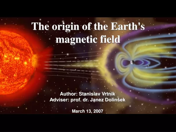
The origin of the Earth's magnetic field Author: Stanislav Vrtnik Adviser: prof. dr. Janez Dolinšek March 13, 2007
Outline 1Introduction 2 Structure of the Earth 3 The self-excited dynamo 4 An Earth-like numerical dynamo models 5 The approaching polarity reversal 6 Conclusions
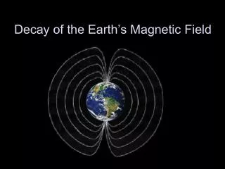
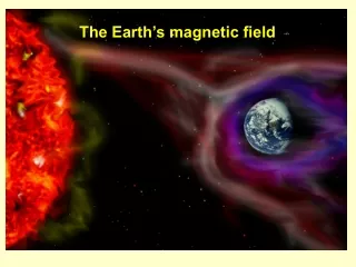
1Introduction Geomagnetic field is generated in Earth’s core Temperatures > 3000 K; above Curie point(Tc(Fe) = 1043 K; Tc(Ni) = 627 K ) Magnetic field is generated by electrical current Unsustained electrical current would dissipate within 20.000 years Paleomagnetic records (ancient field recorded in sediment and lavas ) Earth’s magnetic field exists millions of years Mechanism that regenerates electrical currents (self-excited dynamo) The polarity reversal Earth will lose magnetic shield for high-energy particles
2 Structure of the Earth Not to scale The outercore: 2180 km tick Liquid Fe, Ni, some light elements Theinner core: Radius of 1220 km Solid (Fe, Ni) The mantle: 2900 km thick Silicate rocks (with Fe, Mg) Solid, but ductile can flow on large timescale Convection of the material moves tectonic plates Pressure increase with depth and change viscosity Lower mantle flow less easily The Crust: 5-70 km tick < 1% Earth’s volume 100 millions years old Some grains are 4.4 billion years old Part of the lithosphere divided on tectonic plates Crust Upper mantle Lower mantle Liquid outer core Solid inner core To scale
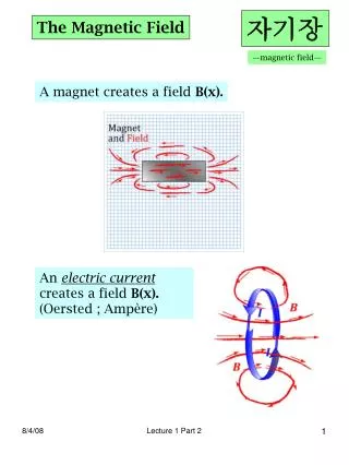
3 The self-excited dynamo Self-excited dynamo model was first proposed by Sir Joseph Larmor in 1919 Magnetic instability →(perturbation of the field is exponentially amplified) Simple experiment with mechanical disk device Magnetic flux through the disk: Induced voltage: Faraday disk dynamo
3 The self-excited dynamo Permanent magnet →replaced with solenoid Magnetic flux through the disk: Induced voltage: Electrical current is given by: Self-excited dynamo R- electrical resistivity of the complete circuit
3 The self-excited dynamo Electrical current is given by: Solution of the differential equation is: System becomes unstable when: (W < WC)the resistivity will damp any initial magnetic perturbation A) (W < WC)the system undergoes a bifurcation →an initial perturbation of the field will be exponentially amplified B)
4 An Earth-like numerical dynamo models Nonlinear three-dimensional model is needed Geodynamo operates in ‘strong field’ regime: nonlinear magnetic Lorentz force ≈ Coriolis force → Lorentz force cannot be treated as perturbation → nonlinear numerical computation is required Cowling’s theorem: self-sustained magnetic field produced by a dynamo cannot be axisymmetric → no 2D solution can be sought → problem has to be investigated directly in 3D
4.1 The magnetohydrodynamics Equations Induction equation: - magnetic field - velocity - the magnetic diffusivity interaction diffusion A) magnetic field decreases exponentially (tEarth = 20.000 years) B) magnetic field is "frozen" into the conducting fluid
4.1 The magnetohydrodynamics Equations Navier-Stokes equation: - mass density - external forces: Lorentz force gravity force Coriolis force buoyancy force - scalar pressure - viscosity To simulate the geodynamo we also need equations for: the gravity potential the heat flow Model for geodynamo can have up to 10 equations
4.2 3D simulation of a geomagnetic field Glatzmaier-Roberts model: with the dimensions, rotate rate, heat flow and the material properties of the Earth’s core Time step: 20 days Simulation now spans more than 300.000 years The simulation took several thousand CPU hours on the Cray C-90 supercomputer Yellow - where the fluid flow is the greatest. The core-mantle boundary - blue the inner core boundary - red G.A. Glatzmaier and P.H. Roberts
4.2 3D simulation of a geomagnetic field • Magnetic field is similar to the Earth's field: • Intensity of the dipole moment • A dipole dominated structure • Westward drift of the non-dipolar field at the surface (0.2° per year) G.A. Glatzmaier & P.H. Roberts
4.2 3D simulation of a geomagnetic field • 36.000 years into the simulation magnetic dipole underwent polarity reversal • over a period of a 1000 years. • the magnetic dipole moment decreases down to 10% • recovered immediately after • consistent with the paleomagnetic records 500 yr before 500 yr after Middle of reversal a) b) c) G.A. Glatzmaier & P.H. Roberts
4.2 3D simulation of a geomagnetic field • The longitudinal average of the 3D magnetic field (out to the surface) • Left – lines of force of the poloidal part of the field • Right – contours of the toroidal part of the field • Red (blue) contours – eastward (westward) directed toroidal field • Green (yellow) lines – clockwise (anticlockwise) poloidal field 5000 yr before Middle of reversal 4000 yr after G.A. Glatzmaier & P.H. Roberts, Nature, 377, 203-209 (1995)
4.2 3D simulation of a geomagnetic field • The radial component of the magnetic field (Hammer projection) • Upper plots (surface); lower plots (core-mantle boundary) • Red (blue) contours represent outward (inward) directed field • Intensity at the surface is multiplied by 10 G.A. Glatzmaier & P.H. Roberts, Nature, 377, 203-209 (1995)
4.2 3D simulation of a geomagnetic field • Rotation of the inner core relative to the surface: • In simulation rotates 2° to 3° per year faster than at the surface • Motivated seismologists to search for evidence (0.3° to 0.5° year faster ) • The field couples the inner core to the eastward flowing fluid • analogous to a synchronous electric motor G.A. Glatzmaier & P.H. Roberts
5 The approaching polarity reversal • Study of the geodynamo has received considerable attention in the press • Concerns of an approaching polarity reversal • The magnetic field protects Earth’s surface from high-energy particles • Sun wind, cosmic rays from deep space • When the field switches polarity, its strength can drop to below 10% • for few 1000 years. • with potentially disastrous consequences for: the atmosphere, the climate and life. • These concerns are supported by observational facts
5 The approaching polarity reversal The dipole moment: • The first term of the spherical harmonic expansion • It can be recovered in the past (paleomagnetic records) • Measurements show rapid and steady decrease • of the geomagnetic dipole moment • Primary motive for pondering the possibility of an • approaching reversal • The geomagnetic field amplitude is a fluctuating quantity • The present dipole moment is still significantly • higher than its averaged value • Over the last polarity interval and the three preceding ones
5 The approaching polarity reversal Direction of the dipole moment: • Tilt angle according to the axis of rotation • The angle is rapidly increasing toward 90° • Opposite of what is expected for a reversal
5 The approaching polarity reversal South North The magnetic dip poles: 1960 • The two places on Earth • Horizontal component of the field is zero • Local objects • They are affected by all components in a • spectral expansion • Move independently of one another 1980 • The northern magnetic dip pole velocity • 40 km/year ( last few years) • 15 km/year (last century) • The southern magnetic dip pole velocity • decreasing (now 10 km/year) • The dip pole is simply an ill defined quantity 2000
5 The approaching polarity reversal The overdue reversal: • The last reversal dates back some 800.000 years • 7 reversal in last 2 million years • The reversal rate is not constant • Average over few million years is 1 per million years • Maximum value is 6 reversals per million years • Maximum: Superchrones (10 millions years)
6 Conclusions • Numerical models are successful but: • restricted to a very remote parameter regime • viscous force is much larger than are in the liquid core • Experimental fluid dynamos were created (1999 in Latvia and Germany) • the flows were extremely confined • Dynamo action works on a large variety of natural bodies • planets in the solar system (Venus and Mars excepted) • Sun (reverses with a relatively regular period of 22 years) • galaxies exhibit their own large-scale magnetic field • Evidence for an imminent reversal remains rather weak • The typical timescale for a reversal is of the order of 1000 years