Ch 6.5: Impulse Functions
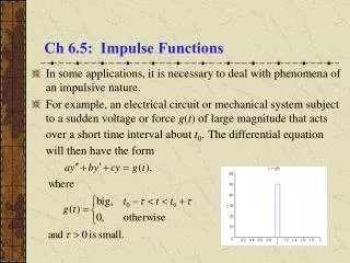
Ch 6.5: Impulse Functions . In some applications, it is necessary to deal with phenomena of an impulsive nature.

Ch 6.5: Impulse Functions
E N D
Presentation Transcript
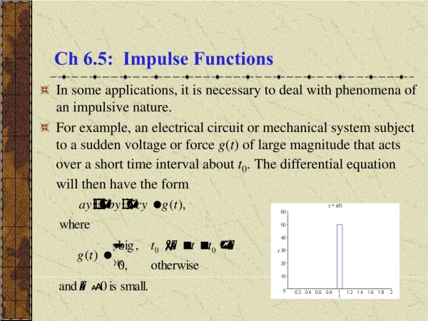
Ch 6.5: Impulse Functions • In some applications, it is necessary to deal with phenomena of an impulsive nature. • For example, an electrical circuit or mechanical system subject to a sudden voltage or force g(t) of large magnitude that acts over a short time interval about t0.The differential equation will then have the form
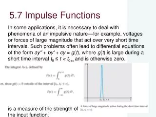
Measuring Impulse • In a mechanical system, where g(t) is a force, the total impulse of this force is measured by the integral • Note that if g(t) has the form then • In particular, if c = 1/(2), then I() = 1 (independent of ).
Unit Impulse Function • Suppose the forcing function d(t) has the form • Then as we have seen, I() = 1. • We are interested d(t) acting over shorter and shorter time intervals (i.e., 0). See graph on right. • Note that d(t) gets taller and narrower as 0. Thus for t 0, we have
Dirac Delta Function • Thus for t 0, we have • The unit impulse function is defined to have the properties • The unit impulse function is an example of a generalized function and is usually called the Dirac delta function. • In general, for a unit impulse at an arbitrary point t0,
Laplace Transform of (1 of 2) • The Laplace Transform of is defined by and thus
Laplace Transform of (2 of 2) • Thus the Laplace Transform of is • For Laplace Transform of at t0= 0, take limit as follows: • For example, when t0= 10, we have L{(t-10)} = e-10s.
Product of Continuous Functions and • The product of the delta function and a continuous function f can be integrated, using the mean value theorem for integrals: • Thus
Example 1: Initial Value Problem (1 of 3) • Consider the solution to the initial value problem • Then • Letting Y(s) = L{y}, • Substituting in the initial conditions, we obtain or
Example 1: Solution (2 of 3) • We have • The partial fraction expansion of Y(s) yields and hence
Example 1: Solution Behavior (3 of 3) • With homogeneous initial conditions at t = 0 and no external excitation until t = 7, there is no response on (0, 7). • The impulse at t = 7 produces a decaying oscillation that persists indefinitely. • Response is continuous at t = 7 despite singularity in forcing function. Since y' has a jump discontinuity at t = 7, y'' has an infinite discontinuity there. Thus singularity in forcing function is balanced by a corresponding singularity in y''.