A Primer on Mixed Integer Linear Programming
A Primer on Mixed Integer Linear Programming. Using Matlab, AMPL and CPLEX at Stanford University Steven Waslander, May 2 nd , 2005. Outline. Optimization Program Types Linear Programming Methods Integer Programming Methods AMPL-CPLEX Example 1 – Production of Goods MATLAB-AMPL-CPLEX

A Primer on Mixed Integer Linear Programming
E N D
Presentation Transcript
A Primer on Mixed Integer Linear Programming Using Matlab, AMPL and CPLEX at Stanford University Steven Waslander, May 2nd, 2005
Outline • Optimization Program Types • Linear Programming Methods • Integer Programming Methods • AMPL-CPLEX • Example 1 – Production of Goods • MATLAB-AMPL-CPLEX • Example 2 – Rover Task Assignment
General Optimization Program • Standard form: • where, • Too general to solve, must specify properties of X, f,g and h more precisely.
Complexity Analysis • (P) – Deterministic Polynomial time algorithm • (NP) – Non-deterministic Polynomial time algorithm, • Feasibility can be determined in polynomial time • (NP-complete) – NP and at least as hard as any known NP problem • (NP-hard) – not provably NP and at least as hard as any NP problem, • Optimization over an NP-complete feasibility problem
Optimization Problem Types – Real Variables • Linear Program (LP) • (P) Easy, fast to solve, convex • Non-Linear Program (NLP) • (P) Convex problems easy to solve • Non-convex problems harder, not guaranteed to find global optimum
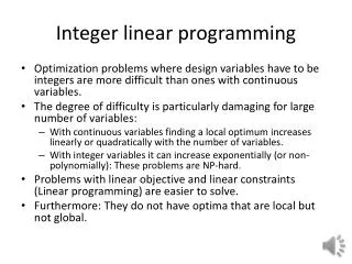
Optimization Problem Types – Integer/Mixed Variables • Integer Programs (IP) : • (NP-hard) computational complexity • Mixed Integer Linear Program (MILP) • Our problem of interest, also generally (NP-hard) • However, many problems can be solved surprisingly quickly! • MINLP, MILQP etc. • New tools included in CPLEX 9.0!
x2 cT x1 Solution Methods for Linear Programs • Simplex Method • Optimum must be at the intersection of constraints (for problems satisfying Slater condition) • Intersections are easy to find, change inequalities to equalities
x2 -cT x1 Solution Method for Linear Programs • Interior Point Methods • Apply Barrier Function to each constraint and sum • Primal-Dual Formulation • Newton Step • Benefits • Scales Better than Simplex • Certificate of Optimality
x1=0 x1=2 x1=1 X2=0 X2=1 X2=2 X2=0 X2=1 X2=2 X2=0 X2=1 X2=2 Solution Methods for Integer Programs • Enumeration – Tree Search, Dynamic Programming etc. • Guaranteed to find a feasible solution (only consider integers, can check feasibility (P) ) • But, exponential growth in computation time
x2 Integer Solution -cT LP Solution x1 Solution Methods for Integer Programs • How about solving LP Relaxation followed by rounding?
x2 -cT x1 Integer Programs • LP solution provides lower bound on IP • But, rounding can be arbitrarily far away from integer solution
x2 x2 -cT -cT x1 x1 Combined approach to Integer Programming • Why not combine both approaches! • Solve LP Relaxation to get fractional solutions • Create two sub-branches by adding constraints x1≥2 x1≤1
LP + x1≤3 + x2≤2 J* = J3 LP + x1≤3 + x2≥3 J* = J4 LP + x1≤3 + x2≥4 J* = J5 LP + x1≥4 + x2≥4 J* = J6 Solution Methods for Integer Programs • Known as Branch and Bound • Branch as above • LP give lower bound, feasible solutions give upper bound LP J* = J0 x1= 3.4, x2= 2.3 LP + x1≤3 J* = J1 LP + x1≥4 J* = J2 x1= 3, x2= 2.6 x1= 3.7, x2= 4
Branch and Bound Method for Integer Programs • Branch and Bound Algorithm 1. Solve LP relaxation for lower bound on cost for current branch • If solution exceeds upper bound, branch is terminated • If solution is integer, replace upper bound on cost 2. Create two branched problems by adding constraints to original problem • Select integer variable with fractional LP solution • Add integer constraints to the original LP 3. Repeat until no branches remain, return optimal solution.
x2 -cT x1 Integer Programs • Order matters • All solutions cause branching to stop • Each feasible solution is an upper bound on optimal cost, allowing elimination of nodes Branch x1 Branch x2 Branch x1 then x2
x2 x1 Additional Refinements – Cutting Planes • Idea stems from adding additional constraints to LP to improve tightness of relaxation • Combine constraints to eliminate non-integer solutions • All feasible integer solutions remain feasible • Current LP solution is not feasible Added Cut
Mixed Integer Linear Programs • No harder than IPs • Linear variables are found exactly through LP solutions • Many improvements to this algorithm are included in CPLEX • Cutting Planes (Gomery, Flow Covers, Rounding) • Problem Reduction/Preprocessing • Heuristics for node selection
Solving MILPs with CPLEX-AMPL-MATLAB • CPLEX is the best MILP optimization engine out there. • AMPL is a standard programming interface for many optimization engines. • MATLAB can be used to generate AMPL files for CPLEX to solve.
Introduction to AMPL • Each optimization program has 2-3 files • optprog.mod: the model file • Defines a class of problems (variables, costs, constraints) • optprog.dat: the data file • Defines an instance of the class of problems • optprog.run: optional script file • Defines what variables should be saved/displayed, passes options to the solver and issues the solve command
Running AMPL-CPLEX on Stanford Machines • Get Samson • Available at ess.stanford.edu • Log into epic.stanford.edu • or any other Solaris machine • Copy your AMPL files to your afs directory • SecureFX (from ess.stanford.edu) sftp to transfer.stanford.edu • Move into the directory that holds your AMPL files • cd ./private/MILP
Running AMPL-CPLEX on Stanford Machines • Start AMPL by typing ampl at the prompt • Load the model file • ampl: model optprog.mod; (note semi-colon) • Load the data file • ampl: data optprog.dat; • Issue solve and display commands • ampl: solve; • ampl: display variable_of_interest; • OR, run the run file with all of the above in it • ampl: quit; • Epic26:~> ampl example.run
Example MILP Problem • Decision on when to produce a good and how much to produce in order to meet a demand forecast and minimize costs • Costs • Fixed cost of production in any producing period • Production cost proportional to amount of goods produced • Cost of keeping inventory • Constraints • Must meet fixed demand vector over T periods • No initial stock • Maximum number of goods, M, can be produced per period
AMPL:Example Model File - Part 1 #------------------------------------------------ #example.mod #------------------------------------------------ # PARAMETERS param T > 0; # Number of periods param M > 0; # Maximum production per period param fixedcost {2..T+1} >= 0; # Fixed cost of production in period t param prodcost {2..T+1} >= 0; # Production cost of production in period t param storcost {2..T+1} >= 0; # Storage cost of production in period t param demand {2..T+1} >= 0; # Demand in period t # VARIABLES var made {2..T+1} >= 0; # Units Produced in period t var stock {1..T+1} >= 0; # Units Stored at end of t var decide {2..T+1} binary; # Decision to produce in period t
AMPL:Example Model File - Part 2 # COST FUNCTION minimize total_cost: sum {t in 2..T+1} (prodcost[t] * made[t] + fixedcost[t] * decide[t] + storcost[t] * stock[t]); # INITIAL CONDITION subject to Init: stock[1] = 0; # DEMAND CONSTRAINT subject to Demand {t in 2..T+1}: stock[t-1] + made[t] = demand[t] + stock[t]; # MAX PRODUCTION CONSTRAINT subject to MaxProd {t in 2..T+1}: made[t] <= M * decide[t];
AMPL: Example Data File #------------------------------------------------ #example.dat #------------------------------------------------ param T:= 6; param demand := 2 6 3 7 4 4 5 6 6 3 7 8; param prodcost := 2 3 3 4 4 3 5 4 6 4 7 5; param storcost := 2 1 3 1 4 1 5 1 6 1 7 1; param fixedcost := 2 12 3 15 4 30 5 23 6 19 7 45; param M := 10;
AMPL:Example Run File #------------------------------------------------ #example.run #------------------------------------------------ model example.mod; data example.dat; solve; display made;
AMPL: Example Results epic26:~/private/example_MILP> ampl example.run ILOG AMPL 8.100, licensed to "stanford-palo alto, ca". AMPL Version 20021031 (SunOS 5.7) ILOG CPLEX 8.100, licensed to "stanford-palo alto, ca", options: e m b q CPLEX 8.1.0: optimal integer solution; objective 212 15 MIP simplex iterations 0 branch-and-bound nodes made [*] := 2 7 3 10 4 0 5 7 6 10 7 0 ;
Using MATLAB to Generate and Run AMPL files • Can auto-generate data file in Matlab • fprintf(fid,['param ' param_name ' := %12.0f;\n'],p); • Use ! command to execute system command, and > to dump output to a file • ! ampl example.run > CPLEXrun.txt • Add printf to run file to store variables for Matlab • In .run: printf: variable > variable.dat; • In Matlab: load variable.dat;
Further Example – Task Assignment • System Goal only: Minimum completion time • All tasks must be assigned • Timing Constraints between tasks (loitering allowed) • Obstacles must be avoided
Task Assignment Difficulties • NP-Hard problem • Instead of assigning 6 tasks, must select from all possible permutations • Even 2 aircraft, 6 tasks yields 4320 permutations • Timing Constraints • Shortest path through tasks not necessarily optimal
Task Assignment:Model File #Objective function minimize cost: ## <-- COST FUNCTION ## #MissionTime; minMaxTimeCostwt * MissionTime + (sum{j in BVARS} costStore[j]*z[j]) + (sum{idxWP in WP, idxUAV in UAV} tLoiter[idxWP,idxUAV]); #Constrain 1 visit per waypoint subject to wpCons {idxWP in WP}: (sum{p in BVARS} (permMat[idxWP,p]*z[p])) = 1; #Constrain 1 permutation per vehicle subject to permCons {idxUAV in UAV}: sum{p in BVARS : firstSlot[idxUAV]<=ord(p) and ord(p)<=lastSlot[idxUAV]} z[p] <= 1; #Constrain "tLoiter{idxWP,idxUAV}" to be 0 if "idxWP" is not visited by "idxUAV" subject to WPandUAV {idxUAV in UAV, idxWP in WP}: tLoiter[idxWP,idxUAV] <= M * sum{p in BVARS: firstSlot[idxUAV]<=ord(p) and ord(p)<=lastSlot[idxUAV]} (permMat[idxWP,p]*z[p]); #Constrain "minMaxTime" to be greater than largest mission time subject to inequCons {idxUAV in UAV}: MissionTime >= (sum{p in BVARS} (minMaxTimeCons[idxUAV,p]*z[p])) # flight time + (sum{idxWP in WP} tLoiter[idxWP,idxUAV]); # loiter time #How long it will loiter at (or just before reaching) idxWP subject to loiteringTime {idxWP in WP}: tLoiterVec[idxWP] = sum{idxUAV in UAV} tLoiter[idxWP,idxUAV]; #Timing Constraints!! subject to timing {t in TCONS}: TOA[timeConstraintWpts[t,2]] >= TOA[timeConstraintWpts[t,1]] + Tdelay[t]; #Constrain "TimeOfArrival" of each waypoint subject to timeOfArrival {idxWP in WP}: TOA[idxWP] = sum{p in BVARS} timeStore[idxWP,p]*z[p] + tLoiterBefore[idxWP]; #Solve for "tLoiterBefore" subject to sumOfLoiteringTime1 {p in BVARS, idxWP in WP}: tLoiterBefore[idxWP] <= sum{idxPreWP in WP} (ord3D[idxWP,idxPreWP,p]*tLoiterVec[idxPreWP]) + M*(1-permMat[idxWP,p]*z[p]); subject to sumOfLoiteringTime2 {p in BVARS, idxWP in WP}: tLoiterBefore[idxWP] >= sum{idxPreWP in WP} (ord3D[idxWP,idxPreWP,p]*tLoiterVec[idxPreWP]) # given a waypoint idxWP and a permutation p, it equals 0 if idxWP is # not visited, equals 1 if it is visited. #Constrain loiterable waypoints subject to constrainLoiter {idxWP in WP, idxUAV in UAV: loiteringCapability[idxWP,idxUAV]==0}: tLoiter[idxWP,idxUAV] = 0; # AMPL model file for UAV coordination given permutations # # timing constraints exist # adjust TOE by loitering at waypoints param Nvehs integer >=1; # number of vehicles, also number of permutations per vehicle constraints param Nwps integer >=1; # number of waypoints, also number of waypoint constraints param Nperms integer >=1; # number of total permutations, also number of binary variables param M := 10000; # large number param Tcons integer; # number of timing constraints set WP ordered := 1..Nwps; set UAV ordered := 1..Nvehs; set BVARS ordered := 1..Nperms ; set TCONS ordered := 1..Tcons; #parameters for permMat*z = 1 param permMat{WP,BVARS} binary; # parameters for minimizing max time param minMaxTimeCons{UAV,BVARS}; # parameters for timing constraint param timeConstraintWpts{TCONS,1..2} integer; param timeStore{WP,BVARS}; param Tdelay{TCONS}; # parameters for calculating loitering time param firstSlot{UAV} integer; # position in the BVARS where permutations for idxUAV begin param lastSlot{UAV} integer; # position in the BVARS where permutations for idxUAV end param ord3D{WP,WP,BVARS} binary; # ord3D{idxWP,idxPreWP,p} # if idxPreWP is visited before idxWP or at the same time as idxWP in permutation p param loiteringCapability{WP,UAV} binary; # =0 if it cannot wait at that WP. # cost weightings param costStore{BVARS}; #cost weighting on binary variables, i.e. cost for each permutation param minMaxTimeCostwt; #cost weighting on variable that minimizes max time for individual missions # decision variables var MissionTime >=0; var z{BVARS} binary; var tLoiter{WP,UAV} >=0; #idxUAV loiters for "tLoiter[idxWP,idxUAV]" on its way to idxWP # intermediate variables var tLoiterVec{WP} >=0; var TOA{WP} >=0; var tLoiterBefore{WP} >=0; #the sum of loitering time before reaching idxWP
Rover Task Assignment:Model File • Set definitions in AMPL • Great for adding collections of constraints # from Task_Assignment.mod param Nvehs integer >=1; param Nwps integer >=1; set UAV ordered := 1..Nvehs; set WP ordered := 1..Nwps; var tLoiter{WP,UAV} >=0; subject to loiteringTime {idxWP in WP}: tLoiterVec[idxWP] = sum{idxUAV in UAV} tLoiter[idxWP,idxUAV];
Further Resources • AMPL textbook • AMPL: A modeling language for mathematical programming, Robert Fourer, David M. Gay, Brian W. Kernighan • CPLEX user manuals • On Stanford network at /usr/pubsw/doc/Sweet/ilog • MS&E 212 class website • Further examples and references • Class Website • This presentation • Matlab libraries for AMPL