Belief Propagation
Belief Propagation. by Jakob Metzler. Outline. Motivation Pearl’s BP Algorithm Turbo Codes Generalized Belief Propagation Free Energies. Probabilistic Inference. From the lecture we know: Computing the a posteriori belief of a variable in a general Bayesian Network is NP-hard

Belief Propagation
E N D
Presentation Transcript
Belief Propagation by Jakob Metzler
Outline • Motivation • Pearl’s BP Algorithm • Turbo Codes • Generalized Belief Propagation • Free Energies
Probabilistic Inference • From the lecture we know: Computing the a posteriori belief of a variable in a general Bayesian Network is NP-hard • Solution: approximate inference • MCMC sampling
Probabilistic Inference • From the lecture we know: Computing the a posteriori belief of a variable in a general Bayesian Network is NP-hard • Solution: approximate inference • MCMC sampling • Belief Propagation
Belief Propagation • In BBNs, we can define the belief BEL(x) of a node x in a graph in the following way: • In BP, the pi and lambda terms are messages sent to the node x from its parents and children, respectively BEL(x) = P(x|e) = P(x|e+,e-) = P(e-|x, e+) * P(x|e+) / P(e-|e+)
Pearl’s BP Algorithm • Initialization • For nodes with evidence e • (xi) = 1 wherever xi= ei ; 0 otherwise • (xi) = 1 wherever xi= ei ; 0 otherwise • For nodes without parents • (xi) = p(xi) - prior probabilities • For nodes without children • (xi) = 1 uniformly (normalize at end)
Pearl’s BP Algorithm 1. Combine incoming messages from all parents U={U1,…,Un} into 2. Combine incoming messages from all children Y={Y1,…Yn} into 3. Compute 4. Send messages to children Y 5. Send messages to parents X
Pearl’s BP Algorithm U1 U2 X Y1 Y2
Pearl’s BP Algorithm U1 U2 X Y1 Y2
Pearl’s BP Algorithm U1 U2 X Y1 Y2
Pearl’s BP Algorithm U1 U2 X Y1 Y2
Pearl’s BP Algorithm U1 U2 X Y1 Y2
Properties of BP • Exact for polytrees • Each node separates Graph into 2 disjoint components • On a polytree, the BP algorithm converges in time proportional to diameter of network – at most linear • Work done in a node is proportional to the size of CPT • Hence BP is linear in number of network parameters • For general BBNs • Exact inference is NP-hard • Approximate inference is NP-hard
Properties of BP • Another example of exact inference: Hidden Markov chains • Applying BP to its BBN representation yields the forward-backward algorithm
Loopy Belief Propagation • Most graphs are not polytrees • Cutset conditioning • Clustering • Join Tree Method • Approximate Inference • Loopy BP
Loopy Belief Propagation • If BP is used on graphs with loops, messages may circulate indefinitely • Empirically, a good approximation is still achievable • Stop after fixed # of iterations • Stop when no significant change in beliefs • If solution is not oscillatory but converges, it usually is a good approximation • Example: Turbo Codes
Outline • Motivation • Pearl’s BP Algorithm • Turbo Codes • Generalized Belief Propagation • Free Energies
Decoding Algorithms • Information U is to be transmitted reliably over a noisy, memoryless channel • U is encoded systematically into codeword X=(U, X1) • X1 is a “codeword fragment • It is received as Y=(Ys, Y1) • The noisy channel has transition probabilities defined by p(y|x) = Pr{Y=y|X=x}
Decoding Algorithms • Since it is also memoryless, we have • The decoding problem: Infer U from observed values Y by maximizing the belief: • If we define the belief is given by
Decoding using BP • We can also represent the problem with a bayesian network: • Using BP on this graph is another way of deriving the solution mentioned earlier.
Turbo Codes • The information U can also be encoded using 2 encoders: • Motivation: using 2 simple encoders in parallel can produce a very effective overall encoding • Interleaver causes permutation of inputs
Turbo Codes • The bayesian network corresponding to the decoding problem is not a polytree any more but has loops:
Turbo Codes • We can still approximate the optimal beliefs by using loopy Belief Propagation • Stop after # of iterations • Choosing the order of belief updates among the nodes derives “different” previously known algorithms • Sequence U->X1->U->X2->U->X1->U etc. yields the well-known turbo decoding algorithm • Sequence U->X->U->X->U etc. yields a general decoding algorithm for multiple turbo codes • and many more
Turbo Codes Summary • BP can be used as a general decoding algorithm by representing the problem as a BBN and running BP on it. • Many existing, seemingly different decoding algorithms are just instantiations of BP. • Turbo codes are a good example of successful convergence of BP on a loopy graph.
Outline • Motivation • Pearl’s BP Algorithm • Turbo Codes • Generalized Belief Propagation • Free Energies
BP in MRFs • BP can also be applied to other graphical models, e.g. pairwise MRFs • Hidden variables xi and xj are connected through a compatibility function • Hidden variables xi are connected to observable variables yi by the local “evidence” function • Pairwise, so it can also be abbreviated as • The joint probability of {x} is given by
BP in MRFs • In pairwise MRFs, the messages & beliefs are updated the following way:
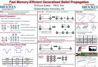
Generalized BP • We can try to improve inference by taking into account higher-order interactions among the variables • An intuitive way to do this is to define messages that propagate between groups of nodes rather than just single nodes • This is the intuition in Generalized Belief Propagation (GPB)
GBP Algorithm 1) Split the graph into basic clusters [1245],[2356], [4578],[5689]
GBP Algorithm 2) Find all intersection regions of the basic clusters, and all their intersections [25], [45], [56], [58], [5]
GBP Algorithm 3) Create a hierarchy of regions and their direct sub-regions
GBP Algorithm 4) Associate a message with each line in the graph e.g. message from [1245]->[25]: m14->25(x2,x5)
GBP Algorithm 5) Setup equations for beliefs of regions - remember from earlier: - So the belief for the region containing [5] is: - for the region [45]: - etc.
GBP Algorithm 6) Setup equations for updating messages by enforcing marginalization conditions and combining them with the belief equations: e.g. condition yields, with the previous two belief formulas, the message update rule
Experiment • [Yedidia et al., 2000]: • “square lattice Ising spin glass in a random magnetic field” • Structure: Nodes are arranged in square lattice of size n*n • Compatibility matrix: • Evidence term:
Experiment Results • For n>=20, ordinary BP did not converge • For n=10: (marginals)
Outline • Motivation • Pearl’s BP Algorithm • Turbo Codes • Generalized Belief Propagation • Free Energies