Download

1 / 27
280 likes | 1.02k Vues
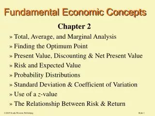
Fundamental Economic Concepts. Chapter 2 Total, Average, and Marginal Finding the Optimum Point Present Value, Discounting & NPV Risk and Uncertainty Risk-Return & Probability Standard Deviation & Coefficient of Variation Expected Utility & Risk-Adjusted Discount Rates Use of a z-value.

E N D
Fundamental Economic Concepts Chapter 2 • Total, Average, and Marginal • Finding the Optimum Point • Present Value, Discounting & NPV • Risk and Uncertainty • Risk-Return & Probability • Standard Deviation & Coefficient of Variation • Expected Utility & Risk-Adjusted Discount Rates • Use of a z-value 2002 South-Western Publishing
How to Maximize Profits • Decision Making Isn’tFree • Max Profit { A, B}, but suppose that we don’t know the Profit {A} or the Profit {B} • Should we hire a consultant for $1,000? • Should we market an Amoretto Flavored chewing gum for adults? • complex combination of marketing, production, and financial issues
Break Decisions Into Smaller Units: How Much to Produce ? profit • Graph of output and profit • Possible Rule: • Expand output until profits turn down • But problem of local maxima vs. global maximum GLOBAL MAX MAX A quantity B
Average Profit = Profit / Q PROFITS • Slope of ray from the origin • Rise / Run • Profit / Q = average profit • Maximizing average profit doesn’t maximize total profit MAX C B profits quantity Q
Marginal Profits = /Q profits max • profits of the last unit produced • maximum marginal profits occur at theinflection point (A) • Decision Rule: produce where marginal profits = 0. C B A Q average profits marginal profits Q
Using Equations • profit = f(quantity) or • = f(Q) • dependent variable & independent variable(s) • average profit =Q • marginal profit = / Q
Optimal Decision (one period)example of using marginal reasoning • The scale of a project should expand until • MB = MC Example: screening for prostate or breast cancer • How often? MC MB frequency per decade
Present Value • Present value recognizes that a dollar received in the future is worth less than a dollar in hand today. • To compare monies in the future with today, the future dollars must be discounted by a present value interest factor, PVIF= 1/(1+i), where i is the interest compensation for postponing receiving cash one period. • For dollars received in n periods, the discount factor is PVIFn =[1/(1+i)]n
Net Present Value • NPV = Present value of future returns minus Initial outlay. • This is for the simple example of a single cost today yielding a benefit or stream of benefits in the future. • For the more general case, NPV = Present value of all cash flows (both positive and negative ones). • NPV Rule: Do all projects that have positive net present values. By doing this, the manager maximizes shareholder wealth. • Some investments may increase NPV, but at the same time, they may increase risk.
Net Present Value (NPV) • Most business decisions are long term • capital budgeting, product assortment, etc. • Objective: max the present value of profits • NPV = PV of future returns - Initial Outlay • NPV = t=0 NCFt / ( 1 + rt )t • where NCFt is the net cash flow in period t • Good projects have • High NCF’s • Low rates of discount
Brand identify and loyalty Control over distribution Patents or legal barriers to entry Superior materials Difficulty for others to acquire factors of production Superior financial resources Economies of large scale or size Superior management Sources of Positive NPVs
Risk and Uncertainty • Most decisions involve a gamble • Probabilities can be known or unknown, and outcomes can be known or unknown • Risk -- exists when: • Possible outcomes and probabilities are known • e.g., Roulette Wheel or Dice • Uncertainty -- exists when: • Possible outcomes or probabilities are unknown • e.g., Drilling for Oil in an unknown field
Concepts of Risk • When probabilities are known, we can analyze risk using probability distributions • Assign a probability to each state of nature, and be exhaustive, so thatpi = 1 States of Nature StrategyRecession Economic Boom p = .30 p = .70 Expand Plant - 40 100 Don’t Expand - 10 50
Payoff Matrix • Payoff Matrix shows payoffs for each state of nature, for each strategy • Expected Value =r= ri pi. • r= ri pi = (-40)(.30) + (100)(.70) = 58 if Expand • r= ri pi = (-10)(.30) + (50)(.70) = 32 if Don’t Expand • Standard Deviation = = (ri - r ) 2. pi ^ ^ ^ ^
Example ofFinding Standard Deviations expand = SQRT{ (-40 - 58)2(.3) + (100-58)2(.7)} = SQRT{(-98)2(.3)+(42)2 (.7)} = SQRT{ 4116} = 64.16 don’t = SQRT{(-10 - 32)2 (.3)+(50 - 32)2 (.7)} = SQRT{(-42)2 (.3)+(18)2 (.7) } = SQRT { 756} = 27.50 Expanding has a greater standard deviation, but higher expected return.
Coefficients of Variationor Relative Risk ^ • Coefficient of Variation (C.V.) = / r. • C.V. is a measure of risk per dollar of expected return. • The discount rate for present values depends on the risk class of the investment. • Look at similar investments • Corporate Bonds, or Treasury Bonds • Common Domestic Stocks, or Foreign Stocks
Projects of Different Sizes: If double the size, the C.V. is not changed!!! Coefficient of Variation is good for comparing projects of different sizes Example of Two Gambles A: Prob X } R = 15 .5 10 } = SQRT{(10-15)2(.5)+(20-15)2(.5)] .5 20 } = SQRT{25} = 5 C.V. = 5 / 15 = .333 B: Prob X } R = 30 .5 20 } = SQRT{(20-30)2 ((.5)+(40-30)2(.5)] .5 40 } = SQRT{100} = 10 C.V. = 10 / 30 = .333
Continuous Probability Distributions (vs. Discrete) • Expected valued is the mode for symmetric distributions A is riskier, but it has a higher expected value B A ^ ^ RB RA
What Went Wrong at LTCM? • Long Term Capital Management was a ‘hedge fund’ run by some top-notch finance experts (1993-1998) • LTCM looked for small pricing deviations between interest rates and derivatives, such as bond futures. • They earned 45% returns -- but that may be due to high risks in their type of arbitrage activity. • The Russian default in 1998 changed the risk level of government debt, and LTCM lost $2 billion
The St. Petersburg Paradox • The St. Petersburg Paradox is a gamble of tossing a fair coin, where the payoff doubles for every consecutive head that appears. The expected monetary value of this gamble is: $2·(.5) + $4·(.25) + $8·(.125) + $16·(.0625) + ... = 1 + 1 + 1 + ... = . • But no one would be willing to wager all he or she owns to get into this bet. It must be that people make decisions by criteria other than maximizing expected monetary payoff.
Utility is “satisfaction” Each payoff has a utility As payoffs rise, utility rises Risk Neutral -- if indifferent between risk & a fair bet Expected Utility Analysisto Compare Risks .5•U(10) + .5•U(20) is a fair bet for 15 U U(15) 10 15 20
Prefer a certain amount to a fair bet Prefer a fair bet to a certain amount Risk Averse Risk Seeking U U certain risky risky certain 10 15 20 10 15 20
Suppose we are given a quadratic utility function: U = .09 X - .00002 X2 Gamble: 30% probability of getting 100; 30% of getting 200; and a 40% probability of getting 400. Versus a certain $150? U(150) = 13.05 (plug X=150 into utility function) Find “Expected Utility” of the gamble EU = pi U(Xi) EU = .30(8.8) + .30(17.2) + .40( 32.8) = 20.92 Expected Utility: an example
Risk Adjusted Discount Rates • Riskier projects should be discounted at higher discount rates • PV = t / ( 1 + k) t where k varies with risk and t are cash flows. • kA > kB as in diagram since A is riskier B A
Market-based rates Look at equivalent risky projects, use that rate Is it like a Bond, Stock, Venture Capital? Capital Asset Pricing Model (CAPM) Project’s “beta” and the market return Sources of Risk Adjusted Discount Rates
z-Values • z is the number of standard deviations away from the mean • z = (r - r )/ • 68% of the time within 1 standard deviation • 95% of the time within 2 standard deviations • 99% of the time within 3 standard deviations Problem:income has a mean of $1,000 and a standard deviation of $500. What’s the chance of losing money? ^
Diversification The expected return on a portfolio is the weighted average of expected returns in the portfolio. Portfolio risk depends on the weights, standard deviations of the securities in the portfolio, and on the correlation coefficients between securities. The risk of a two-security portfolio is: p = (WA2·A2 + WB2·B2 + 2·WA·WB·AB·A·B ) • If the correlation coefficient, AB, equals one, no risk reduction is achieved. • When AB < 1, then p < wA·A + wB·B. Hence, portfolio risk is less than the weighted average of the standard deviations in the portfolio.