Rank-Balanced Trees
Rank-Balanced Trees. Siddhartha Sen, Princeton University WADS 2009 Joint work with Bernhard Haeupler and Robert E. Tarjan . Observation. Computer science is (still) a young field. We often settle for the first (good) solution. It may not be the best: the design space is rich.

Rank-Balanced Trees
E N D
Presentation Transcript
Rank-Balanced Trees Siddhartha Sen, Princeton University WADS 2009 Joint work with Bernhard Haeupler and Robert E. Tarjan
Observation Computer science is (still) a young field. We often settle for the first (good) solution. It may not be the best: the design space is rich.
Research Agenda For fundamental problems, systematically explore the design space to find the best solutions, seeking elegance: “a quality of neatness and ingenious simplicity in the solution of a problem (especially in science or mathematics).” wordnet.princeton.edu/perl/webwn Keep the design simple, allow complexity in the analysis.
Searching: Dictionary Problem Maintain a set of items, so that Access: find a given item Insert: add a new item Delete: remove an item are efficient. Assumption: items are totally ordered, so that binary comparison is possible
Binary Search Tree Symmetric order e > < c i a g n k Why not hashing?
Binary Search Tree e > c i > a g n < k Access k
Binary Search Tree e > c i < a g n > h k Insert h
Binary Search Tree Find successor Swap e Delete c k i k a g n h i k m Delete i
Problem: imbalance How to bound the height? • Maintain local balance condition, rebalance after insert or delete balanced tree • Restructure after each access self-adjusting tree Store balance information in nodes, guarantee O(log n) height After (during) insert/delete, restore balance bottom-up (top-down): • Update balance information • Restructure along access path a b c d e f
Restructuring primitive:(Single) Rotation y x right left x y C A A B B C Preserves symmetric order Changes heights Takes O(1) time
Known Balanced Trees not binary AVL trees (“passé” according to one author) weight balanced trees 2,3 trees B trees red-black trees etc. Goal: small height, little rebalancing, simple algorithms
Ranks Each node has an integer rank, a proxy for height Convention: leaves have rank 0, missing nodes have rank -1 rank of tree = rank of root rank difference of a child = rank of parent - rank of child i-child: node of rank difference i i,j-node: children have rank differences i and j
Example of a rank-balanced tree 3 e c i 2 1 2 1 a g n 1 1 0 1 1 1 h k 1 0 1 0 If all rank differences are positive, rank height
Rank Rules AVL trees: every node is a 1,1- or 1,2-node Rank-balanced trees: every node is a 1,1-, 1,2-, or 2,2-node (rank differences are 1 or 2) Red-black trees: all rank differences are 0 or 1, no 0-child is the parent of another All need one balance bit per node.
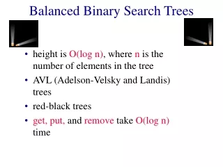
Height bounds nk = minimum n for rank k AVL trees: n0 = 1, n1 = 2, nk = nk-1 + nk-2 + 1, nk = Fk+3 - 1 nk = Fk+3 - 1, Fk+2 < k k log n 1.44lg n Rank-balanced trees: n0 = 1, n1 = 2, nk = 2nk-2, nk = 2k/2 k 2lg n Same bound for red-black trees
Insertion example Demote a a Promote a 1 0 > b Promote b Rotate left at b 1 0 0 1 > c 1 0 0 Insert c Insert b Insert a
Insertion example b Promote b 1 2 > Promote c a c Demote c 1 1 2 1 0 0 0 > Promote d Rotate left at d d 1 0 1 0 > e 1 0 0 Insert c Insert d Insert e
Insertion example b Demote b 2 > a d Rotate left at d Promote d 1 1 2 0 0 2 > c e Promote e 2 1 0 1 0 1 0 > f 0 1 0 Insert f Insert e
Insertion example d 2 b e 1 1 1 1 a f c 1 0 0 1 1 0 Insert f
Rebalancing: insertion Non-terminal 0, 1, or 2 rotations O(log n) rank changes No 2,2 nodes = AVL trees log n height!
Deletion example e d Swap with successor Double demote e 2 Demote b b d f e Delete 1 1 1 0 2 1 a f c 1 0 0 1 1 0 Double rotate at c Double promote c Delete f Delete d Delete a
Deletion example c 2 b e 0 0 2 2 Delete f
Rebalancing: deletion Non-terminal 0, 1, or 2 rotations O(log n) rank changes
Amortized (time-averaged) analysis If ti is the actual time of operation i and i is the potential of the data structure after operation i, the amortized time of operation i is
Non-terminal cases Must decrease potential!
Insertions: 1,1-node 1,2-node Deletions: 2,2-node 1,1- or 1,2-node = #1,1-nodes + 2 #2,2-nodes non-terminating steps are free, last insertion step: Δ 2, last deletion step: Δ 3 If there are m inserts and d deletes (n = m - d), the number of rebalancing steps is O(m + d)
Rank-Balanced Trees height 2lg n 2 rotations per rebalancing O(1) amortized rebalancing time Red-Black Trees height 2lg n 3 rotations per rebalancing O(1) amortized rebalancing time Yes. No. Are rank-balanced trees better?
Better height bound? Sequential Insertions: rank-balanced red-black height = lg n (best) height = 2lg n (worst) Theorem. The height of a rank-balanced tree is at most log m. Degrades gracefully from AVL trees as d/m 1
Proof Give a node a count of 1 when it is inserted Total amount of count in tree is m Potential of a node = total count in its subtree When a node is deleted, its count is added to its parent if it has one Let k be the minimum potential of a node of rank k Claim: ksatisfies 0 = 1, 1 = 2, k = 1 + k-1 + k-2 for k > 1 m Fk+3 - 1 k
Proof of Claim k = 1 + k-1 + k-2 for k > 1 Easy for 1,1- and 1,2-nodes Harder for 2,2-nodes (created by deletions) But counts are inherited
Rebalancing frequency How high does rebalancing propagate? O(m + d) rebalancing steps total, which implies O((m + d) / k) insertions/deletions at rank k Actually, we can show: Theorem. There are O((m + d)/2k/3) rebalancing steps at rank k.
Proof Use an exponential potential: 1,1- and 2,2-nodes of rank i get potential bi 1,2-nodes of rank i get potential bi-2 where b = 21/3 The potential change in the non-terminal steps telescopes. Combine this effect with initialization and terminal step.
Telescoping potential = -bi+3 … bi+2 - bi+3 1 0 bi+1 - bi+2 0 1 2 1 bi - bi+1 0 0 1 2 1 bi-1 - bi 1 0 1 2 1 1 2 0 …
Fix k. Cut off growth in potential at rank k: 1,1- and 2,2-nodes of rank i: bmin{i,k-3} 1,2-nodes of rank i: bmin{i-2,k-3} Then a rebalancing that propagates to rank k or above decreases the potential by bk-3. The same idea works for red-black trees (we think).
Conclusion Rank-balanced trees are a relaxation of AVL trees with behavior at least as good as red-black trees and better in important ways. Especially the height bound of min{2lg n, log m} Exponential potential functions yield new insights into the efficiency of rebalancing. We anticipate more applications.
Is rebalancing necessary? For insertions, yes. But what about deletions? Deletion rebalancing is complicated, ignored by textbooks, and many database systems do not do it So, can we avoid deletion rebalancing? Yes. Relaxation of AVL trees, ravl trees, achieves log m access time using lglg m + 1 balance bits … and no rebalancing during deletion!