The Use of Mathematica in Control Engineering
700 likes | 1.04k Vues
The Use of Mathematica in Control Engineering. Neil Munro Control Systems Centre UMIST Manchester, England. Linear Model Descriptions Linear Model Transformations Linear System Analysis Tools Design/Synthesis Techniques Pole Assignment Model-Reference Optimal Control

The Use of Mathematica in Control Engineering
E N D
Presentation Transcript
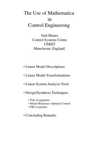
The Use of Mathematica inControl Engineering Neil Munro Control Systems Centre UMIST Manchester, England. • Linear Model Descriptions • Linear Model Transformations • Linear System Analysis Tools • Design/Synthesis Techniques • Pole Assignment • Model-Reference Optimal Control • PID Controller • Concluding Remarks
Linear Model Descriptions • The Control System Professional currently provides • several ways of describing linear system models; e.g. • For systems described by the state-space equations where y is a vector of the system outputs u is a vector of the system inputs and x is a vector of the system state-variables • For systems described by transfer-function relationships where s is the complex variable
Examples: - ss = StateSpace[{{0, 0, 1, 0},{0, 0, 0, 1}, {-(a b), 0, a+b, 0},{0, -(a b), 0, a+b}}, {{0, 0},{0, 0},{1, 0},{0, 1}},{{-b, -a, 1, 1}}]
New Data Formats have been implemented, for these objects, which are fully editable, as follows: - ss = StateSpace[{{0, 0, 1, 0},{0, 0, 0, 1}, {-(a b), 0, a+b, 0},{0, -(a b), 0, a+b}}, {{0, 0},{0, 0},{1, 0},{0, 1}},{{-b, -a, 1, 1}}] now results in the composite data matrix
tfsys = TransferFunction[s, {{((s+2)(s+3))/(s+1)^2,1/(s+1)^2}, {(s+2)/(s+1)^2,(s+1)/((s+1)^2(s+3))}, {1/(s+2),1/(s+1)}}] which now yields
New Data Objects • Four new data objects have been introduced; namely, • Rosenbrock’s system matrix in polynomial form • Rosenbrock’s system matrix in state-space form • The right matrix-fraction description of a system • The left matrix-fraction description of a system.
The system matrix in polynomial form provides a compact description of a linear dynamical system described by arbitrary ordered differential equations and algebraic relationships, after the application of the Laplace transform with zero initial conditions; namely where , u and y are vectors of the Laplace transformed system variables. This set of equations can equally be written as
The system matrix in polynomial form is then defined as When a system matrix in polynomial form is being created, it is important to note that the dimension of the square matrix T(s) must be adjusted to be r, where r is the degree of Det[T(s)]. If the system description is known in state-space form then a special form of the system matrix can be constructed, known as the system matrix in state-space form, as shown below
Matrix Fraction Forms • Given a system description in transfer function matrix form G(s), for certain analysis and design purposes; e.g. the H- approach to robust control system design; it is often convenient to express this model in the form of a left or right matrix-fraction description; e.g. • A left matrix-fraction form of a given transfer function matrix G(s) might be • 2 A right matrix fraction form of a given transfer function matrix G(s) might be
Linear Model Transformations G(s) [A, B, C, D] G(s) System Matrix P(s) in polynomial form G(s) System Matrix P(s) in state-space form [A, B, C, D] System Matrix P(s) in polynomial form [T(s),U(s),V(s),W(s)] Least Order P1(s) P2(s)
New Data Transformations All data formats are fully editable tfsys = TransferFunction[s, {{((s+2)(s+3))/(s+1)^2,1/(s+1)^2}, {(s+2)/(s+1)^2,(s+1)/((s+1)^2(s+3))}, {1/(s+2),1/(s+1)}}] ss = StateSpace[tfsys] rff =RightMatrixFraction[tfsys] rff = RightMatrixFraction[ss,s]
New Data Transformations tfsys = TransferFunction[s, {{(s+1)/(s^2+2s+1)},{(s+2)/(s+1)}}] ps = SystemMatrix[tfsys,TargetFormRightFraction] rff = RightMatrixFraction[ps] TransferFunction[%] ps = SystemMatrix[tfsys,TargetForm LeftFraction] lf = LeftFractionForm[ ]
New Data Transformations tfsys =TransferFunction[s, {{(s+1)/(s^2+2s+1)},{(s+2)/(s+1)}] rff = RightMatrixFraction[tfsys] dt = ToDiscreteTime[tfsys,Sampled->20]//Simplify
New Data Transformations RightMatrixFraction[%] SystemMatrix[dt,TargetForm->RightFraction] SystemMatrix[dt]
A Least-Order form of a System-Matrix in polynomial form is one in which there are no input-decoupling zeros and no output-decoupling zeros, and would yield a minimal state-space realization, when directly converted to state-space form. For example, the polynomial system matrix is not least order, since T(s) and U(s) have 3 input-decoupling zeros at s = {0, 0, -1}; i.e. [T(s) U(s)] has rank 4 at these values of s.
System Analysis Controllable[ss] Observable[ss] ss =[A, B, C, D] Controllable[ps] Observable[ps] Controllable[ps] Observable[ps] MatrixLeftGCD[T(s) U(s)] MatrixRightGCD[T(s) V(s)] SmithForm[T(s) U(s)] McMillanForm[G(s)] Decoupling Zeros Decoupling Zeros
Controllability and Observability In the same way that the controllability and observability of a system described by a set of state space equations can be determined in the Control System Professional by entering the commands Controllable[ss] and Observable[ss] where ss is a StateSpace object. These tests can now also be directly applied to a system matrix object by entering the commands Controllable[sm] and Observable[sm] where sm is a SystemMatrix object in either polynomial form or state space form.
Preliminary Analysis • Reduction of State-Space Equations • Given a system matrix in state-space form • then an input-decoupling zeros algorithm, • implemented in Mathematica, reduces P(s) to • The completely controllable part is then given by
Gasifier Model Format A is 25 x 25 B is 25 x 6 C is 4 x 25 D is 4 x 6 Inputs:- 1 char 2 air 3 coal 4 steam 5 limestone 6 upstream disturbance Outputs:- 1 gas cv 2 bed mass 3 gas pressure 4 gas temperature
Preliminary Analysis The original 25th order system is numerically very ill conditioned. The eigenvalues cover a significant range in the complex plane, ranging from -0.00033 to -33.1252. The condition number is 5.24 x 10¹⁹. At w = 0 the maximum and minimum singular values are 147500 and 50, respectively. The Kalman controllability and observability tests yield a rankof 1, and the controllability and observability gramians are :-
Preliminary Analysis Application of the decoupling zeros algorithm to [sI-A, B] yielded Dimensions of Dimensions of Dimensions of indicating that the system had 7 input-decoupling zeros, which was confirmed by transforming A and B to spectral form.
Smith and McMillan Forms The Smith form of a polynomial matrix and the McMillan form of a rational polynomial matrix are both important in control systems analysis. Consider an x m polynomial matrix N(s), then the Smith form of N(s) is defined as S(s) = L(s)N(s)R(s) and L(s) and R(s) are unimodular matrices.
Smith and McMillan Forms Consider now an x m rational polynomial matrix G(s), and let G(s) = N(s)/d(s) where d(s) is the monic least common denominator of G(s), then the McMillan form of G(s) is defined as where M(s) is the result of dividing the Smith form of N(s) by d(s), and cancelling out all common factors
Design Methods Synthesis Methods Pole Assignment PID Controller Optimal Control Nyquist Array Model Ref. Opt. Control Robust NA Model-Order Reduction Nonlinear Systems
Design/Synthesis Methods Methods implemented are:- 1 Pole Assignment - Some Observations 2 Model-Reference Optimal Control 3 The Systematic Design of PID Controllers 4 Uncertain Nonlinear Systems 5 Robust Direct Nyquist Array Design Method 6 Model-Order Reduction
Pole Assignment • We consider four main types of approaches • ACKERMANN’S FORMULA • SPECTRAL APPROACH • MAPPING APPROACH • EIGENVECTOR METHODS Control Systems Centre - UMIST
Ackermann’s Formula Here is the controllability matrix of [A,b], and pc(s) is the desired closed-loop system characteristic polynomial. Spectral Approach where Here, i and i are the open-loop system and desired closed-loop system poles, respectively, and the vi´ are the associated reciprocal eigenvectors. Control Systems Centre - UMIST
Mapping Approach The state-feedback matrix is given as where is the controllability matrix of [A, b] Here, the ai and i are the coefficients of the open-loop and closed-loop system characteristic polynomials, respectively. Control Systems Centre - UMIST
Eigenvector Methods It is also possible to determine the state-feedback pole assignment compensator as where the mi are randomly chosen scalars and the uciare the closed-loop system eigenvectors calculated from Selecting mi =1, for example, the state-feedback compensator can be found as Control Systems Centre - UMIST
Comparison of Dyadic Methods under Numeric Considerations Control Systems Centre - UMIST
Comparison of Dyadic Methods under Symbolic Considerations Control Systems Centre - UMIST
Model-Reference Optimal Control Model Reference LQR System The resulting optimal feedback controller Ko can be partitioned as where K11 and K21 operate on the reference-model state vector xM and K12 and K22 operate on the system state vector x.
Model Reference LQR feedback paths. Model Reference LQR System Closed-Loop.
Unit-step on reference input 1 Unit-step on reference input 2 Unit-step on reference input 3 Unit-step on reference input 4
The PID Controller • In recent years, several researchers have been re-examining the PID controller to determine the limiting Kp, Ki, and Kd parameter values to guarantee a stable closed-loop system; namely, • Keel and Bhattacharyya • Ho, Datta, and Bhattacharyya • Shafei and Shenton • Astrom and Hagglund • Munro and Soylemez
Test compensator arrangement Test compensator space
The Nyquist plot for Kp = 0.5 and Ki = 0.5 The admissible PI compensator space
Stability Performance Robustness Simplicity Transparency increasing difficulty Design Requirements
Acknowledgements My thanks to Dr Igor Bakshee of Wolfram Research for his interest and help in carrying out this work.
Control Systems Centre UMIST D-Stability = Sin() Im D Re d
Control Systems Centre UMIST The Nyquist Plot Approach • Here, we detect 5 axis crossings, (-2,+2,+2,-1,-1), where the last is due to the infinite arc, on the right, due to the pole at the origin.
The Nyquist Plot Approach The resulting stability boundary is Note that the origin is not included in the region because the basic system is unstable.
Control Systems Centre UMIST The Nyquist Plot Approach • Here, with Kp = 5 and Ki = 18 the system is stable, even with an additional gain of k =1.3134 • yielding closed-loop poles = • -0.2519 ± 5.4879i • -1.2320 ± 1.5258i • -0.0161 ± 0.4510i
Diagonal Dominance Concepts Various definitions of Diagonal Dominance exist, namely :- Rosenbrock’s row/column form ~ R Limebeer’s Generalised Diagonal Dominance ~ L Bryant & Yeung’s Fundamental Dominance ~ Y where the conservatism of the resulting dominance criterionreduces as Y < L < R Mathematica Code