AVL Trees
AVL Trees. Outline. Background Define balance Maintaining balance within a tree AVL trees Difference of heights Rotations to maintain balance. Background. From previous lectures: Binary search trees store linearly ordered data Best case height: Q (ln( n ))

AVL Trees
E N D
Presentation Transcript
Outline Background Define balance Maintaining balance within a tree • AVL trees • Difference of heights • Rotations to maintain balance
Background From previous lectures: • Binary search trees store linearly ordered data • Best case height: Q(ln(n)) • Worst case height: O(n) Requirement: • Define and maintain a balance to ensure Q(ln(n)) height
Prototypical Examples These two examples demonstrate how we can correct for imbalances: starting with this tree, add 1:
Prototypical Examples This is more like a linked list; however, we can fix this…
Prototypical Examples Promote 2 to the root, demote 3 to be 2’s right child, and 1 remains the left child of 2
Prototypical Examples The result is a perfect, though trivial tree
Prototypical Examples Alternatively, given this tree, insert 2
Prototypical Examples Again, the product is a linked list; however, we can fix this, too
Prototypical Examples Promote 2 to the root, and assign 1 and 3 to be its children
Prototypical Examples The result is, again, a perfect tree These examples may seem trivial, but they are the basis for the corrections in the next data structure we will see: AVL trees
AVL Trees We will focus on the first strategy: AVL trees • Named after Adelson-Velskii and Landis Balance is defined by comparing the height of the two sub-trees of a node • An empty tree has height –1 • A tree with a single node has height 0
AVL Trees A binary search tree is said to be AVL balanced if: • The difference in the heights between the left and right sub-trees is at most 1, and • Both sub-trees are themselves AVL trees
AVL Trees AVL trees with 1, 2, 3, and 4 nodes:
AVL Trees Here is a larger AVL tree (42 nodes):
AVL Trees The root node is AVL-balanced: • Both sub-trees are of height 4:
AVL Trees All other nodes (e.g., AF and BL) are AVL balanced • The sub-trees differ in height by at most one
Height of an AVL Tree By the definition of complete trees, any complete binary search tree is an AVL tree Thus an upper bound on the number of nodes in an AVL tree of height h a perfect binary tree with 2h + 1 – 1 nodes • What is an lower bound?
Height of an AVL Tree Let F(h) be the fewest number of nodes in a tree of height h From a previous slide: F(0) = 1 F(1) = 2 F(2) = 4 Can we find F(h)?
Height of an AVL Tree The worst-case AVL tree of height h would have: • A worst-case AVL tree of height h – 1on one side, • A worst-case AVL tree of height h – 2 on the other, and • The root node We get: F(h) = F(h – 1) + 1+ F(h – 2)
Height of an AVL Tree This is a recurrence relation: The solution?
Height of an AVL Tree Use Maple: > rsolve( {F(0) = 1, F(1) = 2, F(h) = 1 + F(h - 1) + F(h - 2)}, F(h) ); > asympt( %, h );
Height of an AVL Tree This is approximately F(h) ≈ 1.8944 f h where f≈1.6180 is the golden ratio • That is, F(h) = W(f h) Thus, we may find the maximum value of h for a given n: logf( n / 1.8944 ) = logf( n ) – 1.3277
Height of an AVL Tree In this example, n = 88, the worst- and best-case scenarios differ in height by only 2
Height of an AVL Tree If n = 106, the bounds on h are: • The minimum height: log2( 106 ) – 1 ≈ 19 • the maximum height : logf( 106 / 1.8944 ) < 28
Maintaining Balance To maintain AVL balance, observe that: • Inserting a node can increase the height of a tree by at most 1 • Removing a node can decrease the height of a tree by at most 1
Maintaining Balance Insert either 15 or 42 into this AVL tree
Maintaining Balance Inserting 15 does not change any heights
Maintaining Balance Inserting 42 changes the height of two of the sub-trees
Maintaining Balance To calculate changes in height, the member function must run in O(1) time Our implementation of height is O(n): template <typename Comp> int Binary_search_node<Comp>::height() const { return max( ( left() == 0 ) ? 0 : 1 + left()->height(), ( right() == 0 ) ? 0 : 1 + right()->height() ); }
Maintaining Balance Introduce a member variable int tree_height; The member function is now: template <typename Comp> int BinarySearchNode<Comp>::height() const { return tree_height; }
Maintaining Balance Only insert and erase may change the height • This is the only place we need to update the height • These algorithms are already recursive
Insert template <typename Comp> void AVL_node<Comp>::insert( const Comp & obj ) { if ( obj < element ) { if ( left() == 0 ) { left_tree = new AVL_node<Comp>( obj ); tree_height = 1; } else { left()->insert( obj ); tree_height = max( tree_height, 1 + left()->height() ); } } else if ( obj > element ) { // ... } }
Maintaining Balance Using the same, tree, we mark the stored heights:
Maintaining Balance Again, consider inserting 42 • We update the heights of 38 and 44:
Maintaining Balance If a tree is AVL balanced, for an insertion to cause an imbalance: • The heights of the sub-trees must differ by 1 • The insertion must increase the height of the deeper sub-tree by 1
Maintaining Balance Starting with our sample tree
Maintaining Balance Inserting 23: • 4 nodes change height
Maintaining Balance Insert 9 • Again 4 nodes change height
Maintaining Balance In both cases, there is one deepest node which becomes unbalanced
Maintaining Balance Other nodes may become unbalanced • E.g., 36 in the left tree is also unbalanced We only have to fix the imbalance at the lowest point
Maintaining Balance Inserting 23 • Lowest imbalance at 17 • The root is also unbalanced
Maintaining Balance A quick rearrangement solves all the imbalances at all levels
Maintaining Balance Insert 31 • Lowest imbalance at 17
Maintaining Balance A simple rearrangement solves the imbalances at all levels
Maintaining Balance: Case 1 Consider the following setup • Each blue triangle represents a tree of height h
Maintaining Balance: Case 1 Insert ainto this tree: it falls into the left subtree BLof b • Assume BL remains balanced • Thus, the tree rooted at b is also balanced
Maintaining Balance: Case 1 However, the tree rooted at node fis now unbalanced • We will correct the imbalance at this node
Maintaining Balance: Case 1 We will modify these three pointers • At this point, this references the unbalanced root node f
Maintaining Balance: Case 1 Specifically, we will rotate these two nodes around the root: • Recall the first prototypical example • Promote node b to the root and demote node fto be the right child ofb AVL_node<Comp> *pl = left(), *BR = left()->right();