Frequency: Number of times event occurs Proportion: Frequency / Total n (0≤PROP. ≤1 ) Percent: 100 * Proportion Ratio

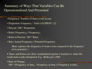
1. Summary of Ways That Variables Can Be Operationalized And Presented • Frequency: Number of times event occurs • Proportion: Frequency / Total n (0≤PROP. ≤1) • Percent: 100 * Proportion • Ratio: Frequency1 / Frequency2 • Ratio in Percent: 100 * Ratio • Rate: Actual Frequency / Potential Frequency • (Rate captures the frequency of some event compared to the frequency of its potential. ) • Rates and Ratios are often standardized against a baseline to make the result more easily interpreted. E.g., Births per 1,000 • Rate of Change: 100 * (Frequency at time2 - Frequency at time1)/ Frequency at time1

2. We now know how to organize the data to describe its general characteristics. We can describe measures of central tendency and distributions of our variables. Next, we want to begin to look at the relationships between variables. We have made hypotheses about the expected relationships and we will learn how to test those hypotheses. Before that, we can begin to see the relationships in tabular and graphical form. The central point is to show how the breakdown of the dependent variable varies with different values of one or more independent variables.

3. RELATIONS AMONG VARIABLES A variable is a characteristic of a person, place or thing.For people we often look at such variables as their gender, race, religion, PID. For places, perhaps, the percent urban, crime rate, number of calories consumed per day. When, say, we want to compare the behavior of men to women or compare crime in one city to another, or ask why questions, such as: Why do some people vote, while others do not? Why do some people join extremist groups, others not? We are asking about the relationship between variables. Today, we’ll focus on looking at the relationship between nominal variables, that is, relations between categorical variables.

4. Remember: Nominal, also called CATEGORICAL VARIABLES, are used simply to group people. E.G., categorize them by gender [M,F], or Religious Affiliation [P,C,J,M, H], Party ID [R,I,D], etc. Group people into categories that have no numerical meaning. Once they are grouped, we can compare their values for other variables. If we hypothesize that the outcomes of some variable, Y, depend on the categories of some variable, X, we can begin to evaluate our hypothesis using a table.

5. Remember: The dependent variable is the response variable, measuring the behavior we want to understand. The independent variable is the explanatory or predictor variable that is hypothesized to influence our dependent variable. The dependent variable changes in response to changes in the independent variable. It predicts change on the dependent variable. I D or X Y The arrow indicates the hypothesized direction of the predicted relationship. The independent variable comes before, occurs earlier in time, is perhaps a causal variable, whereas a dependent variable means the effect. Some change in the environment or in the individual is related to a change in behavior.

6. Tables • One way to describe relationships is with tables. Tables depict relationships between variables. The simplest table depicts the relationship between onedependent variable and one independent variable. • One dependent variable of interest to political scientists studying elections is vote choice: Some people vote for the Democratic candidate, other people vote for the Republican. • Every election year the NES draws a representative sample of the American electorate to study voting behavior. All told about 1500 people are randomly sampled and interviewed. • Let's treat whether a citizen voted for Dole or Clinton in the 1996 presidential election as our dependent variable.

8. Basic Rules for Constructing and Interpreting Crosstabulations • Determine the title: Write a clear description in which the Dependent Variable comes first, then the Independent Variable(s). EG, "1996 Presidential Vote by Gender" Reader should be able to tell what is being compared without reading the accompanying text. Here we are looking at vote choice as a function of gender. 2. Next, Determine categories for the Dep and Ind Vars, here Vote Dole or Clinton. Vote choice is a (categorical) dichotomous variable. The Ind Var can also be broken down as a dichotomy -- Male or Female, producing a 2 by 2 table, with each "cell" -- a, b, c, or d -- showing the number of people in each category. 3. Next, Label the Columns and Rows. Here is a key question. Which should be the column variable, which the row? By convention the Independent variable (Gender) is the column variable. The DV makes up the rows – with title on left. 4. Next Important decision: Which way to calculate percentages.

11. Reading and Interpreting Tables Crosstabs with Controls

12. CONTROLLING for a THIRD VARIABLE • Main effects: Partisanship, Income, & Gender (each of the factors influenced vote choice ) • Concept called “control variables” will help us answer an important question: How do the different independent variables interact? • Interactions: Gender and Party ID Gender and income Party ID and income

16. Effects of Controlling for a Third Variable: four possibilities when controlling for a 3rd Variable • The independent effect is maintained • The now you see it now you don’t effect • Something from nothing effect • The stretch and shrink effect

17. The Independent Effect Maintained:

19. Now you see it now you don’t effect

21. Something from Nothing Effect

23. The Stretch and Shrink Effect

26. Whatever the mean – as long as the distribution is normally distributed -- and whatever the sd the 68-95-99.7 rule applies -- 68%, two-thirds of all the cases fall within + 1 sd of the mean, 95% of the cases within 2 sd of the mean, and 99.7% of the cases are within + 3 sd of the mean. • The more "peaked" the distribution the smaller the sd, but still, half the cases fall above the mean, half below. • So, sometimes the distance between 1 sd and the mean is wide; there is a lot of variability around the center; whereas at other times the range is narrow. • But what is important here is that although the means of different distributions may differ, as well as the sd of the distributions, IF the distribution is normally distributed -- that is, symmetrical and single peaked -- we can describe the distributions in terms of a “standard normal distribution” , and use the 68-95-99.7 percent rule to talk about thetypicality or extremity of scores -- where exactly a score is located in a NDC.

27. Computing Probabilities from NDC • What is the probability of a score greater than 1 standard deviation above the mean? • + 1 sd: p = .68. • Half of .68: p = .34 • Plus .50 from the other half: • .50 + .34 = .84 • And finally …

28. where The Standardized Score or Z-score Z is defined for a population as and X is any raw score. For samples the Z-score is: Σ

29. Z Score • Z score is defined as the number of standard units any score or value is from the mean. • Z score states how many standard deviations the observation X falls away from the mean and in which direction – plus or minus. • What you are doing is dividing the total amount of dispersion in a set of scores by the sd of the distribution mean.