Download
1 / 32
320 likes | 446 Vues
Climatological Aspects of Ice Storms in the Northeastern U.S. Christopher M. Castellano, Lance F. Bosart, and Daniel Keyser Department of Atmospheric and Environmental Sciences University at Albany, State University of New York, Albany, NY John Quinlan and Kevin Lipton

E N D
Climatological Aspects of Ice Storms in the Northeastern U.S. Christopher M. Castellano, Lance F. Bosart, and Daniel Keyser Department of Atmospheric and Environmental Sciences University at Albany, State University of New York, Albany, NY John Quinlan and Kevin Lipton NOAA/NWS/WFO Albany, NY 46th CMOS Conference 25th AMS Conference on Weather Analysis and Forecasting 1 June 2012, Montreal, QC NOAA/CSTAR Grant: NA01NWS4680002
Motivation • Ice storms endanger human life and safety, undermine public infrastructure, and disrupt local and regional economies • Ice storms present a major operational forecast challenge • Ice storms are historically most prevalent and destructive in the northeastern U.S.
Motivation Fig 2. Changnon (2003). The amount of loss (millions of dollars expressed in 2000 values) from ice-storm catastrophes in each climate region during 1949–2000. Values in parentheses are the average losses per catastrophe. Fig 3. Changnon (2003). The number of ice-storm catastrophes in each climate region during 1949–2000. Values in parentheses are those catastrophes that only occurred within the region.
Objectives • Establish a climatology (1993–2010) of ice storms in the northeastern U.S. • Determine environments conducive to ice storms and dynamical mechanisms responsible for freezing rain • Provide forecasters with greater situational awareness of synoptic and mesoscale processes that influence the evolution of ice storms
Data and Methodology Ice Storm Climatology • Identified ice storms using NCDC Storm Data: • Any event listed as an “Ice Storm” • Any event with freezing rain resulting in significant ice accretion (≥ 0.25 in) • Any event with damage attributed to ice accretion • Classified individual ice storms by size:
Geographical Domain CAR BTV GYX BUF ALY BGM BOX CLE CTP PBZ OKX PHI LWX RLX
Data and Methodology Composite Analysis • Identified 35 ice storms impacting WFO Albany’s CWA • Created synoptic composite maps from 2.5° NCEP/NCAR reanalysis data • Generated a composite cross-section using 0.5° CFSR (Climate Forecast System Reanalysis) data • Performed analyses at t−48 h, t−24 h, t = 0
Ice Storms by Season N = 136 Mean = 8
Ice Storms by Month N = 136
Ice Storms by Size N = 136
500-hPa geopotential height (black contours, every 6 dam) and anomalies (shaded, every 30 m) N = 35 t – 48 h
500-hPa geopotential height (black contours, every 6 dam) and anomalies (shaded, every 30 m) N = 35 t – 24 h
500-hPa geopotential height (black contours, every 6 dam) and anomalies (shaded, every 30 m) N = 35 t = 0
850–700-hPa layer wind (arrows, m s-1), 850–700-hPa layer 0°C isotherm (dashed contour), precipitable water (green contours, every 4 mm), and standardized precipitable water anomalies (shaded, every 0.5 σ) N = 35 t – 48 h
850–700-hPa layer wind (arrows, m s-1), 850–700-hPa layer 0°C isotherm (dashed contour), precipitable water (green contours, every 4 mm), and standardized precipitable water anomalies (shaded, every 0.5 σ) N = 35 t – 24 h
850–700-hPa layer wind (arrows, m s-1), 850–700-hPa layer 0°C isotherm (dashed contour), precipitable water (green contours, every 4 mm), and standardized precipitable water anomalies (shaded, every 0.5 σ) N = 35 t = 0
300-hPa wind speed (shaded, every 5 m s-1), 1000–500-hPa thickness (dashed contours, every 6 dam), and mean sea-level pressure (solid contours, every 4 hPa) N = 35 t – 48 h
300-hPa wind speed (shaded, every 5 m s-1), 1000–500-hPa thickness (dashed contours, every 6 dam), and mean sea-level pressure (solid contours, every 4 hPa) N = 35 t – 24 h
300-hPa wind speed (shaded, every 5 m s-1), 1000–500-hPa thickness (dashed contours, every 6 dam), and mean sea-level pressure (solid contours, every 4 hPa) N = 35 t = 0
300-hPa wind speed (shaded, every 5 m s-1), 1000–500-hPa thickness (dashed contours, every 6 dam), and mean sea-level pressure (solid contours, every 4 hPa) N = 35 A A’ t = 0
Frontogenesis [shaded, every 1 K (100 km)-1 (3 h)-1], potential temperature (black, every 2 K), wind speed (green, every 5 m s-1), vertical velocity (dashed red, every 5 μb s-1), and ageostrophic circulation (arrows) N = 35 A A′ 5 m s−1 5 cm s−1
Frontogenesis [shaded, every 1 K (100 km)-1 (3 h)-1], potential temperature (black, every 2 K), wind speed (green, every 5 m s-1), vertical velocity (dashed red, every 5 μb s-1), and ageostrophic circulation (arrows) N = 35 Thermally direct jet entrance region A A′ 5 m s−1 5 cm s−1
Frontogenesis [shaded, every 1 K (100 km)-1 (3 h)-1], potential temperature (black, every 2 K), wind speed (green, every 5 m s-1), vertical velocity (dashed red, every 5 μb s-1), and ageostrophic circulation (arrows) N = 35 Thermally direct jet entrance region Ageostrophic northerlies A A′ 5 m s−1 5 cm s−1
Frontogenesis [shaded, every 1 K (100 km)-1 (3 h)-1], potential temperature (black, every 2 K), wind speed (green, every 5 m s-1), vertical velocity (dashed red, every 5 μb s-1), and ageostrophic circulation (arrows) N = 35 Thermally direct jet entrance region Ageostrophic northerlies Intensifying warm front A A′ 5 m s−1 5 cm s−1
Frontogenesis [shaded, every 1 K (100 km)-1 (3 h)-1], potential temperature (black, every 2 K), wind speed (green, every 5 m s-1), vertical velocity (dashed red, every 5 μb s-1), and ageostrophic circulation (arrows) N = 35 Thermally direct jet entrance region Sloped ascent Ageostrophic northerlies Intensifying warm front A A′ 5 m s−1 5 cm s−1
Frontogenesis [shaded, every 1 K (100 km)-1 (3 h)-1], potential temperature (black, every 2 K), wind speed (green, every 5 m s-1), vertical velocity (dashed red, every 5 μb s-1), and ageostrophic circulation (arrows) N = 35 Thermally direct jet entrance region Sloped ascent Ageostrophic northerlies Intensifying warm front A A′ 5 m s−1 5 cm s−1
Summary: Ice Storm Climatology • Ice storms are climatologically favored between Dec and Mar • Ice storm occurrence is modulated by synoptic and mesoscale topographic features, and proximity to large bodies of water • Ice storms are primarily governed by mesoscale dynamics, but we cannot ignore synoptic–mesoscale linkages
Summary: Composite Analysis • Ice storms are coincident with an amplifying ridge along the East Coast and an upstream trough across the central U.S • Ice storms occur near the equatorward entrance region of an upper-level jet • Ice storms are accompanied by low-to-midlevel moisture transport and warm-air advection via deep southwesterly flow • Ice storms typically occur within a region of enhanced ageostrophic northerlies on the poleward side of a warm front
Thank You! Contact: ccastellano@albany.edu Website: http://www.atmos.albany.edu/student/ccastell