Download
1 / 32
320 likes | 401 Vues
Learn about Fourier series in trigonometric, harmonic, and exponential forms, Laplace and Fourier transforms, line spectra, and spectral envelopes. Understanding integral transforms and Fast Fourier Transform usage. Practice with complex exponentials.

E N D
ECEN3513 Signal AnalysisLecture #9 11 September 2006 • Read section 2.7, 3.1, 3.2 (to top of page 6) • Problems: 2.7-3, 2.7-5, 3.1-1
ECEN3513 Signal AnalysisLecture #10 13 September 2006 • Read section 3.4 • Problems: 3.1-5, 3.2-1, 3.3a & c • Quiz 2 results: Hi = 10, Low = 5.5, Ave = 7.88Standard Deviation = 1.74
Generating a Square Wave... 1.5 0 -1.5 1.0 0 5 cycle per second square wave.
1.5 0 -1.5 1.0 0 1.5 0 -1.5 1.0 0 Generating a Square Wave... 1 vp 5 Hz 1/3 vp 15 Hz
Generating a Square Wave... 1.5 5 Hz+ 15 Hz 0 -1.5 1.0 0 1.5 1/5 vp 25 Hz 0 -1.5 1.0 0
Generating a Square Wave... 5 Hz+ 15 Hz + 25 Hz 1.5 0 -1.5 1.0 0 1.5 1/7 vp 35 Hz 0 -1.5 1.0 0
Generating a Square Wave... 5 Hz+ 15 Hz + 25 Hz + 35 Hz 1.5 0 -1.5 1.0 0 cos2*pi*5t - (1/3)cos2*pi*15t + (1/5)cos2*pi*25t - (1/7)cos2*pi*35t) 5 cycle per second square wave generated using 4 sinusoids
Generating a Square Wave... 1.5 0 -1.5 1.0 0 5 cycle per second square wave generated using 50 sinusoids.
Generating a Square Wave... 1.5 0 -1.5 1.0 0 5 cycle per second square wave generated using 100 sinusoids.
∞ n=1 x(t) periodic T = period ω0 = 2π/T Fourier Series(Trigonometric Form) • x(t) = a0 + ∑ (ancos nω0t + bnsin nω0t) • a0 = (1/T) x(t)1 dt • an = (2/T) x(t)cos nω0t dt • bn = (2/T) x(t)sin nω0t dt T T T
∞ n=1 x(t) periodic T = period ω0 = 2π/T Fourier Series(Harmonic Form) • x(t) = a0 + ∑ cncos(nω0t - θn) • a0 = (1/T) x(t)1 dt • cn2 = an2 + bn2 • θn = tan-1(bn/an) T
∞ n= -∞ T x(t) periodic T = period ω0 = 2π/T Fourier Series(Exponential Form) • x(t) = ∑ dne jnω0t • dn = (1/T) x(t)e-jnω0t dt
Transforms ∞ Laplace X(s) = x(t) e-st dt 0- ∞ X(3) = x(t) e-3t dt 0-
∞ Fourier X(f) = x(t) e-j2πft dt -∞ Transforms • e-j2πft = cos(2πft) - j sin(2πft) • Re[X(f)] = similarity between cos(2πft) & x(t) • Re[X(10.32)] = amount of 10.32 Hz cosine in x(t) • Im[X(f)] = similarity between sin(2πft) & x(t) • -Im[X(10.32)] = amount of 10.32 Hz sine in x(t)
Fourier Series • Time Domain signal must be periodic • Line Spectra • Energy only at discrete frequenciesFundamental (1/T Hz)Harmonics (n+1)/T Hz; n = 1, 2, 3, ... • Spectral envelope is based on FT of periodic base function
∞ ∞ Forward Inverse X(f) = x(t) e-j2πft dt x(t) = X(f) ej2πft df -∞ -∞ Fourier Transforms
∞ ∞ Forward Inverse X(ω) = x(t) e-jωt dt x(t) = X(ω) ejωt dω 2π -∞ -∞ Fourier Transforms
Fourier Transforms • Basic Theory • How to evaluate simple integral transforms • How to use tables • On the job (BS signal processing or Commo) • Mostly you’ll use Fast Fourier TransformInfo above will help you spot errors • Only occasionally will you find FT by handMasters or PhD may do so more often
n = 0 ∑e-jn2πf/T n = 0 Summing Complex Exponentials(T = 0.2 seconds) 1 5 10 15 0 f (Hz)
n = +1 ∑e-jn2πf/T n = -1 Summing Complex Exponentials(T = 0.2 seconds) 3 5 10 15 0 f (Hz)
n = +5 ∑e-jn2πf/T n = -5 Summing Complex Exponentials(T = 0.2 seconds) 11 5 10 15 0 f (Hz)
n = +10 ∑e-jn2πf/T n = -10 Summing Complex Exponentials(T = 0.2 seconds) 21 5 10 15 0 f (Hz)
n = +100 ∑e-jn2πf/T n = -100 Summing Complex Exponentials(T = 0.2 seconds) 201 5 10 15 0 f (Hz)
n = +100 ∑e-jn2πf/T n = -100 Summing Complex Exponentials(T = 0.2 seconds) 20 2.5 5 f (Hz)