GIS for Regional CO2 Source-Sink Matching Optimization
10 likes | 110 Vues
Explore case studies applying GIS to assess CCS potential in California and Texas, optimizing CO2 transportation and injection costs through a least-cost matching model.

GIS for Regional CO2 Source-Sink Matching Optimization
E N D
Presentation Transcript
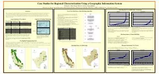
Case Studies for Regional Characterization Using a Geographic Information System Weifeng Li1, Henry Zhang1, Howard J. Herzog1, Richard Rhudy2 1 Laboratory for Energy and the Environment, Massachusetts Institute of Technology, Cambridge, MA 02139; 2 EPRI, 3412 Hillview Ave., Palo Alto, CA 94303 Matching Sources to EOR Sinks (Continued) Least-Cost Path Source-Sink Matching Algorithm Overview This poster presents two case studies of the application of a Geographic Information System (GIS) for the regional characterization of CO2 capture and storage (CCS) potentials. The geographic areas studied are California and eastern Texas. In each case, we evaluated the large concentrated CO2 sources and the storage capacity of geologic formations. Then, we applied our transportation cost model to construct the aggregate transportation cost layer for each region. Finally, we applied our least-cost source-sink matching model to build a CSS network in the study region that minimizes the cumulative CO2 transport and injection cost of the system. California Eastern Texas • The least-cost source-sink matching methodology approximates the optimal source-sink allocation among a set of CO2 sources and CO2 sinks within the study region. • The method links each CO2 source to a least-cost geological sink based on sum of the transportation cost and the injection cost subject to the sink’s storage capacity constraint. • The linking analysis is conducted in two stages. An iterative algorithm presented in the right flow chart is applied in each stage. • In the first stage, the candidate sink set includes only EOR sites where storage projects that transport CO2 to site can earn EOR credits. • If there are sources that remain unmatched or are matched with transportation costs greater than the EOR credits, a second stage analysis will be conducted to link them to non-EOR sinks. • Large Stationary CO2 Sources • Capacity of Geologic Formations Table 1 CO2 Flow Rate by Plant Types, California Potential Sink List and Capacity: California Oil fields with EOR potential 3.2 Gt Non-EOR sinks Non-EOR oil fields 0.2 Gt Gas fields 1.4 Gt Saline aquifers not available Table 2 CO2 Flow Rate by Plant Types, eastern Texas Figure 4 Marginal Transportation Cost in Oil Fields with EOR Potential Table 3 Estimated Relative Construction Cost Factor • Twenty nine sources were matched to EOR sinks, 101 sources remained unmatched in the first stage. • All the transportation costs for matched sources were below the EOR credit value, suggesting that none of the matched sources would enter the Second stage matching. • All of the 31 CO2 sources can be connected to their corresponding EOR sinks in the first stage. • Four sources had transportation costs to the closest EOR site greater than the EOR credit value ($16/t CO2). These sources would be considered in the second stage matching. • Potential Sink List and Capacity: eastern Texas • Oil fields with EOR potential 1.2 Gt • Non-EOR sinks • Gas fields 1.7 Gt • Saline aquifers 196 Gt Matching Sources to Non-EOR Sinks • The CO2 emissions were estimated assuming an operation capacity of 80% for power plants and full production capacity for non-power stationary CO2 sources. The capture efficiency was assumed to be 90% for non-pure CO2 sources and 100% for pure CO2 sources. • We restricted CO2 sources to power plants with design capacity greater than 100 MWe and non-power CO2 sources with the 25-year emissions over 20 Mt in California or 5 Mt in eastern Texas. • The screening criteria: (1) Depth > 800 m; (2) Storage capacity greater than 20 Mt in California or storage capacity greater than 5 Mt in eastern Texas California Eastern Texas • A new round of source-sink matching was applied for the four sources with transportation cost over EOR credit from the first stage. • A final check was run to conduce a full-cost comparison to decide whether they should be matched to EOR or non-EOR sinks. • Except for the source with transportation to EOR site of $16.8/t CO2 that remained to be connected to its EOR destination, the other three sources were reassigned to saline aquifers instead because of the lower full cost. • The second stage source-sink matching was run for the 101 unmatched CO2 sources to link them to non-EOR sinks. • All of the 101 sources were linked to gas fields or saline aquifers. CO2 Pipeline Transportation Cost • Pipelines are considered the most economical means of transporting large quantities of CO2 from the sources to the corresponding sinks. • The pipeline construction costs vary considerably according to local terrains, number of crossings (waterway, railway, highway), and the traversing of populated places, wetlands, and national or state parks. • In order to account for such obstacles, the locations and characteristics of these obstacles were loaded into the GIS database and were used to construct a single aggregate transportation obstacle layer (cost surface). • The transportation cost layer was used to determine the least cost pipeline path for connecting each source and sink. Figure 2 Least-Cost Source-Sink Matching Iterative Algorithm Marginal Abatement Cost Curves Matching Sources to EOR Sinks • CO2 sources linked to EOR sinks: full sequestration cost = capture cost + transport cost – EOR credit • CO2 sources linked to non-EOR sinks: full sequestration cost = capture cost + transport cost + injection cost Eastern Texas California Figure 5 Marginal Abatement Cost Curves • The marginal costs of sequestering 20, 40, or 80 Mt of CO2 per year would be $31/t CO2, $35/t CO2, or $50/t CO2, respectively. • The marginal costs of sequestering 20, 100, or 200 Mt of CO2 per year would be $16/t CO2, $33/t CO2, or $43/t CO2, respectively. • Sequestration costs could be negative for certain ammonia and gas processing plants that have low transportation costs since their capture costs would be less than the assumed EOR credit. Figure 3 CO2 Sources Matching to Oil Fields with EOR Potential in California and Eastern Texas Figure 1 Terrain Maps in California and Eastern Texas


![Geographic Information System [GIS]](https://cdn2.slideserve.com/5315378/geographic-information-system-gis-dt.jpg)