Download

1 / 40
400 likes | 617 Vues
Evaluating an estimated new Keynesian small open economy model. Malin Adolfson , Stefan Laséen , Jesper Lindé, Mattias Villani. Marc Goñi – 19 th April. Introduction Model Methodology Results Conclusion. Motivation.

E N D
Evaluating an estimated new Keynesian small open economy model MalinAdolfson, Stefan Laséen, Jesper Lindé, MattiasVillani Marc Goñi – 19 thApril
IntroductionModel MethodologyResultsConclusion Motivation During the last years, the use of DSGE models for forecasting and policy recommendations has grown. However, key macroeconomic series aren’t still fitted: • Persistence and volatility of real exchange rate • International transmission of business cycles This paper estimates a NK small open economy for Sweden using Bayesian techniques and accounting for the Swedish monetary policy regime shift. By modifying the UIP condition the model is able to account for realistic persistence and volatility of the exchange rate.
IntroductionModel MethodologyResultsConclusion Literature Review Christiano et al (2005) “Nominal rigidities and the dynamic effects of a shock to monetary policy” Smets and Wouters (2003) “An estimated DSGE for the Euro Area” Smets and Wouters (2004) “Forecasting with a BDSGE model. An application to the Euro area” Adolfson et al (2007) “Forecasting performance of an open economy DSGE model with incomplete pass through”
IntroductionModel MethodologyResultsConclusion Outline 1. Model Modified UIP Monetary Policy regime shift 2. Methodology Estimate the DSGE model using Bayesian techniques Use Del Negro, Schorfheide (2004), Del Negro (2007) for misspecification evaluation 3. Results Posterior probabilities and Impulse Responses Forecasting ability Misspecification
IntroductionModelMethodologyResultsConclusion Firms • Domestic Goods Firms The domestic final good is a composite of intermediate goods produced using capital K and labor H subject to price stickyness and an externally financed wage bill. Moreover, it is exposed to technology shock.
IntroductionModelMethodologyResultsConclusion Firms • Final Domestic Good • Intermediate Domestic Good Demand
IntroductionModelMethodologyResultsConclusion Firms • Production Function • Marginal Cost
IntroductionModelMethodologyResultsConclusion Firms • Optimization problem • Phillips Curve for the domestic Goods Sector
IntroductionModelMethodologyResultsConclusion Firms 2. Import and Export Sector The are import consumption and investment firms and export firms Each firm buys the homogeneous foreign (home) good at price P* (Pd) and converts it to a differentiated good through brand naming technology Nominal rigidities in the local currency price imply short run incomplete pass-through
IntroductionModelMethodologyResultsConclusion Firms • Final Import (Export) Good • Intermediate Good Demand • Production function
IntroductionModelMethodologyResultsConclusion Firms • Marginal Cost for the importing firms for the exporting firm • Optimization problem • Phillips curves for Consumption and Investment Imports and Exports
IntroductionModelMethodologyResultsConclusion Households The economy is populated with a continuum of Households which attain utility from consumption, leisure and real cash balances. To purchase these commodities they invest in physical capital and supply capital and labor to firms
IntroductionModelMethodologyResultsConclusion Households • Preferences where,
IntroductionModelMethodologyResultsConclusion Households • Capital Accumulation where,
IntroductionModelMethodologyResultsConclusion Households • Labor Decision
IntroductionModelMethodologyResultsConclusion Households • Bond Holdings The choice between domestic and Foreign bonds balances into a no arbitrage condition (UIP). - Nominal interest rate difference equals expected change in exchange rate Not much empirical support for UIP: - Persistent hump-shaped response of the exchange rate to monetary shock Introduce negative correlation between expected change in exchange rate and risk premium to get this persistence (forward premium puzzle)
IntroductionModelMethodologyResultsConclusion Households • Bond Holdings • Risk Premium • MUIP
IntroductionModelMethodologyResultsConclusion Central Bank As Sweden went from a fixed to a floating exchange rate in 1992 we need to account for this break • Pre 1992 Generalized Taylor Rule
IntroductionModelMethodologyResultsConclusion Central Bank • Post 1992 Allow for three different policy specifications and let the data tell the most appropriate. • Fixed exchange rate rule • Semi-Fixed exchange rate rule
IntroductionModelMethodologyResultsConclusion Central Bank • Inflation Targeting with parameters that is, no break in the monetary policy.
IntroductionModelMethodologyResultsConclusion Shocks where
IntroductionModelMethodologyResultsConclusion Government The Government spends resources in consuming the domestic good, collects taxes from households and transfers the surplus/deficit plus the seigniorage to the households via lump sum taxes
IntroductionModelMethodologyResultsConclusion Foreign Economy Foreign prices, output and interest rate are exogenously given by a 4-lag VAR estimated using un-informative priors
IntroductionModelMethodologyResultsConclusion Model Solution To solve the model consider the market clearing conditions To compute the equilibrium decision rules, • Stationarize all variables • Log linearize around the steady state • Use the AIM algorithm to calculate the numerical reduced form solution
IntroductionModel MethodologyResultsConclusion Data Use quarterly Swedish data for the period 1980Q1-2004Q4 For the foreign variables weight Sweden’s 20 largest trading partners in 1991 according to IMF
IntroductionModel MethodologyResultsConclusion Bayesian Estimation Previously, compute the reduced form solution Construct the observed data vector Transform the reduced form solution into a state-space representation mapping the unobserved state variables to the observed data
IntroductionModel MethodologyResultsConclusion Bayesian Estimation 1. Prior Distribution Set priors for unobserved state variables using 1980Q1-1985Q4 a training sample For the majority of the estimated parameters, use Adolfson et al (2007) Set some priors (stickiness and markup shocks) based on micro evidence and on educated guesses Set identical priors for the parameters in the monetary policy rule (allows to compare them disregarding any “prior” effect)
IntroductionModel MethodologyResultsConclusion Bayesian Estimation 2. Likelihood function To compute the Likelihood function apply the Kalman filter to the state space transformation of the reduced form solution The structural shocks and the exogenous fiscal al foreign VAR shocks enter in such a way that there is no singularity of the Likelihood function
IntroductionModel MethodologyResultsConclusion Bayesian Estimation 3. Posterior distribution Obtain the joint posterior distribution in two steps: • The posterior mode and the Hessian matrix (evaluated at the mode) is computed by standard numerical routines • This Hessian is used in a Metropolis Hastings algorithm to generate a sample for the posterior distribution
IntroductionModel MethodologyResultsConclusion Bayesian Estimation Notes • Calibrate those parameters suspicious of weak identification • Work with a large number of variables to facilitate Identification of parameters and shocks
IntroductionModel MethodologyResultsConclusion Misspecification Following Del Negro, Schorfheide (2004), Del Negro (2007) • Estimate a more flexible empirically oriented VAR with a prior centered at the DSGE with tightness • Find the optimal (maximum likelihood) • If the is large, that is the DSGE-prior pushes the VAR towards the implied cross-equation restrictions, then the model is compatible with the data and, thus, the DSGE is well specified
IntroductionModel MethodologyResultsConclusion Posterior Distribution Table 1 • Monetary policy rules Taylor based rule with a break in parameters gets the best fit Evidence for a break but not for a strong fix exchange rate policy • Parameters In general, similar parameter estimation across specification Wage stickiness and lagged inflation response equal the prior Policy rule parameters similar in the two regimes
IntroductionModel MethodologyResultsConclusion Posterior Distribution • UIP Condition Need to separately identify the risk premium shock from its propagartion Modifying the UIP condition allows to generate the desired exchange rate persistence
IntroductionModel MethodologyResultsConclusion Impulse Responses
IntroductionModel MethodologyResultsConclusion Forecasting Performance
IntroductionModel MethodologyResultsConclusion Forecasting Performance
IntroductionModel MethodologyResultsConclusion Forecasting Performance
IntroductionModel MethodologyResultsConclusion Model Misspecification
IntroductionModel MethodologyResultsConclusion Model Misspecification
IntroductionModel MethodologyResultsConclusion Conclusions • Improve the NK small open economy model by modifying the UIP condition • By improving the acknowledgement of the workings of the economy the CB is now able to derive policy implications a part from forecasting • However, it seems that misspecification should be more considered