Download
1 / 30
300 likes | 372 Vues
Predicting Future Potential Climate-Biomes for the Yukon, Northwest Territories, and Alaska. Goals.

E N D
Predicting Future Potential Climate-Biomes for the Yukon, Northwest Territories, and Alaska
Goals 1) Develop climate-based land-cover categories (cliomes) for Alaska and western Canada using down-scaled gridded historic climate data from the Scenarios Network for Alaska and Arctic Planning (SNAP) and cluster analysis 2) Link the resulting cliomes to land cover classes, and define each biome by both climate and ecosystem characteristics. 3) Couple these cliomes with SNAP’s climate projections, and create predictions for climate-change-induced shifts in cliome ranges and locations. 4) Use the results to identify areas within Alaska, the Yukon and NWT that are least likely to change, and those that are most likely to change over the course of this century.
BackgroundFollow-up to Connecting Alaska Landscapes into the Future Project • Broader spatial scope • More input data • Clustering methodology 3
Improvements over Phase I • Extended scope to northwestern Canada • Used all 12 months of data, not just 2 • Eliminated pre-defined biome/ecozone categories in favor of model-defined groupings (clusters) • Eliminates false line at US/Canada border • Creates groups with greatest degree of intra-group similarity and inter-group dissimilarity • Gets around the problem of imperfect mapping of vegetation and ecosystem types • Allows for comparison and/or validation against existing maps of vegetation and ecosystems
Sampling Extent Area of Canada selected for cluster analysis. Selected area is lightly shaded, and the unselected area is blue. The red line includes all ecoregions that have any portion within NWT. Limiting total area improves processing capabilities.
Methods: SNAP climate models SNAP is a collaborative network of the University of Alaska, state, federal, provincial, and local agencies, NGOs, and industry partners. Its mission is to provide timely access to scenarios of future conditions in Alaska and the Arctic for more effective planning by decision-makers, communities, and industry.
Calculated concurrence of 15 models with data for 1958-2000 for surface air temperature, air pressure at sea level, and precipitation Used root-mean-square error (RMSE) evaluation to select the 5 models that performed best for Alaska and northwestern Canada Focused on A1B, B1, and A2 emissions scenarios Downscaled course resolution GCM data to 2km SNAP data based on CRU historical datasets and IPCC Global Circulation (GCM) models GCM output (ECHAM5) Figure 1A from Frankenberg st al., Science, Sept. 11, 2009
Historical Climate Trends:Ice Breakup Data Ice breakup dates for the Tanana (left) and Yukon (right) Rivers for the full recorded time periods. Days are expressed as ordinal dates. A statistically significant trend toward earlier thaw dates can be found for both rivers.
Methods: cluster analysis • Cluster analysis is the statistical assignment of a set of observations into subsets so that observations in the same cluster are similar in some sense. • It is a method of “unsupervised learning” – where all data are compared in a multidimensional space and classifying patterns are found in the data. • Clustering is common for statistical data analysis and is used in many fields. Example of a dendrogram. Clusters can be created by cutting off this tree at any vertical level, creating (in this case) from one to 29 clusters.
Methods: Partitioning Around Medoids (PAM) • The dissimilarity matrix describes pairwise distinction between objects. • The algorithm PAM computes representative objects, called medoidswhose average dissimilarity to all the objects in the cluster is minimal • Each object of the data set is assigned to the nearest medoid. • PAM is more robust than the well-known kmeans algorithm, because it minimizes a sum of dissimilarities instead of a sum of squared Euclidean distances, thereby reducing the influence of outliers. • PAM is a standard procedure
Resolution limitations • For Alaska, Yukon, and BC, SNAP uses 1961-1990 climatologies from PRISM, at 2 km • For all other regions of Canada SNAP uses climatologies from CRU, at 10 minutes lat/long (~18.4 km) • In clustering these data, the differences in scale and gridding algorithms led to artificial incongruities across boundaries. • The solution was to cluster across the whole region using CRU data, but to project future climate-biomes using PRISM, where available, to maximize resolution and sensitivity to slope, aspect, and proximity to coastlines. CRU data and SNAP outputs after PRISM downscaling
How many clusters? Sample cluster analysis showing 5 clusters, based on CRU 10’ climatologies. This level of detail was deemed too simplistic to meet the needs of end users. • Choice is mathematically somewhat arbitrary, since all splits are valid • Some groupings likely to more closely match existing land cover classifications • How many clusters are defensible? • How large a biome shift is “really” a shift from the conservation perspective? Sample cluster analysis showing 30 clusters, based on CRU 10’ climatologies. This level of detail was deemed too complex to meet the needs of end users, as well as too fine-scale for the inherent uncertainties of the data.
How many clusters? Mean silhouette width for varying numbers of clusters between 3 and 50. High values in the selected range between 10 and 20 occur at 11, 17, and 18.
Eighteen-cluster map for the entire study area. This cluster number was selected in order to maximize both the distinctness of each cluster and the utility to land managers and other stakeholders.
Cluster certainty based on silhouette width. Note that certainty is lowest along boundaries.
Describing the clusters: temperature Mean seasonal temperature by cluster. For the purposes of this graph, seasons are defined as the means of 3-months periods, where winter is December, January, and February, spring is March, April, May, etc.
Describing the clusters:precipitation Precipitation by cluster. Mean annual precipitation varies widely across the clustering area, with Cluster 17 standing out as the wettest. Cluster 17
Describing the clusters:growing degree days, season length, and snowfall Length of above-freezing season and GDD by cluster. Days above freezing were estimated via linear interpolation between monthly mean temperatures. Growing degree days (GDD) were calculated using 0°C as a baseline. Warm-season and cold-season precipitation by cluster. The majority of precipitation in months with mean temperatures below freezing is assumed to be snow (measured as rainwater equivalent).
Describing the clusters: existing land classification Created 2/4/11 3:00 PM by Conservation Biology Institute http://land cover.usgs.gov/nalcms.php GlobCover 2009 North American Land Change Monitoring System (NALCMS 2005) Alaska Biomes and Canadian Ecoregions. AVHRR Land cover, 1995
Comparison of cluster-derived cliomes with existing land cover designations. This table shows only the highest-percentage designation for each land cover scheme. Color-coding helps to distinguish categories.
Baseline maps Modeled cliomes for the historical baseline years, 1961-1990. As in all projected maps, Alaska and the Yukon are shown at 2km resolution based on PRISM downscaling, and the Northwest Territories are shown at 18.4 km resolution based on CRU downscaling.
Future Projections Original 18 clusters Projected cliomes for the five-model composite, A1B (mid-range ) climate scenario. Alaska and the Yukon are shown at 2km resolution and NWT at 10 minute lat/long resolution .
Future Projections 2000’s 2000’s Projected cliomes for the A2 emissions scenario. This scenario assumes higher concentrations of greenhouse gases, as compared to the A1B scenario. 2030’s 2030’s Projected cliomes for the B1 emissions scenario. This scenario assumes lower concentrations of greenhouse gases, as compared to the A1B scenario. 2060’s 2060’s 2090’s 2090’s
Future Projections Original 18 clusters Projected cliomes for single models. The five GCMs offer differing projections for 2090.
Future Projections Projected change and resilience under three emission scenarios. These maps depict the total number of times models predict a shift in cliome between the 2000’s and the 2030’s, the 2030’s and the 2060’s, and the 2060’s and the 2090’s. Note that number of shifts does not necessarily predict the overall magnitude of the projected change.
Discussion: Interpreting results • Comparison with existing land cover designations • Assessment of which shifts are most significant in terms of vegetation communities • Linkages with species-specific research • Habitat characteristics/requirements • Dispersal ability • Historical shifts Dominant AVHRR land cover types by cluster number. All land cover categories that occur in 15% or more of a given cluster are included.
Discussion: Real-world limitations of modeled results • Changes are unlikely to happen smoothly and spontaneously, and are certainly not going to happen instantly • Seed dispersal takes time • Changes to underlying soils and permafrost take even longer • In many cases, intermediate stages are likely to occur when climate change dictates the loss of permafrost , a new forest type, or new hydrologic conditions • Even in cases when biomes do shift on their own, they almost never do so as cohesive units • Trophic mismatches are likely • Invasive species may have greater dispersal abilities than native ones • It may become increasingly difficult to even define what an “invasive species” is
Discussion: Management implications • Identification of refugia • Identification of vulnerable species/areas • Collaboration and dialogue between modelers and field researchers • Selecting focus of future research • Shift from “preservation” to “adaptation” Toolik Lake Catherine Campbell http://www.polartrec.com/expeditions/changing-tundra-landscapes/journals/2008-07-22 Brian Bergamaschi (USGS) sampling wells at Bonanza Creek LTER site. http://hydrosciences.colorado.edu/research/govt_partners.php
Accessing project documents and data • All project inputs and outputs are available to the public • The final report (full report, main text only, or appendices only) can be downloaded here: http://www.snap.uaf.edu/project_page.php?projectid=8 • Maps and data are also available in GIS formats; contact SNAP for further information (nlfresco@alaska.edu)
Acknowledgments The US portion of this study was made possible by the US Fish and Wildlife Service, Region 7, on behalf of the Arctic Landscape Conservation Cooperative (LCC), with Karen Murphy as project lead and assistance from Joel Reynolds and Jennifer Jenkins (USFWS). The Canadian portion of this study was made possible by The Nature Conservancy Canada, Ducks Unlimited Canada, Government Canada and Government Northwest Territories, with Evie Whitten as project lead. Data and analysis were provided by the University of Alaska Fairbanks (UAF) Scenarios Network for Alaska and Arctic Planning (SNAP) program and Ecological Wildlife Habitat Data Analysis for the Land and Seascape Laboratory (EWHALE) lab, with Nancy Fresco, Michael Lindgren, and Falk Huettmann as project leads. Further input was provided by stakeholders from other interested organizations. We would also like to acknowledge the following organizations and individuals: • Karen Clyde, Government YTDavid Douglas, US Geological Survey • Evelyn Gah, Government NWT • Lois Grabke, Ducks Unlimited Canada • Troy Hegel, Government YT • James Kenyon, Ducks Unlimited CanadaWendy Loya , the Wilderness Society • Lorien Nesbitt , Déline Renewable Resources Council • Thomas Paragi, Alaska Department of Fish and Game • Michael Palmer, TNCScott Rupp , SNAPBrian Sieben, Government NWTStuart Slattery, Ducks Unlimited CanadaJim Sparling, Government NWT