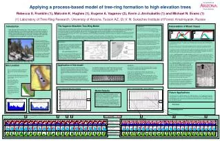
Applying a process-based model of tree-ring formation to high elevation trees

1. Applying a process-based model of tree-ring formation to high elevation trees Rebecca S. Franklin (1), Malcolm K. Hughes (1), Eugene A. Vaganov (2), Kevin J. Anchukaitis (1) and Michael N. Evans (1) (1) Laboratory of Tree-Ring Research, University of Arizona, Tucson AZ, (2) V. N. Sukachev Institute of Forest, Krasnoyarsk, Russia Interpretation of Model Output High elevation bristlecone pines (Pinus longaeva) such as those in the White Mountains of California provide multi-millennial records of growth of great potential value to the reconstruction of past climate. Is it possible to disentangle the influences of temperature and water availability on tree-ring growth in such high, cool, dry places? The Vaganov-Shashkin Tree-Ring Model Introduction Cambial Block In the cambial block, which simulates the growth and formation of wood cells in the tree cambium, the daily growth rate is used to calculate the cellular growth rate V (j,t): V(j,t) = f{j,G(t)} Where theindex j indicates the position in the cambial zone of the growing cell, and V(j,t)is the dependence of growth rate, G(t), on position (Fig 3). Each cell is permitted to be dormant, grow, divide and/or differentiate into xylem on an intra-day interval. If cellular growth rate is greater that Vcr (dormant) but less than position-dependant minimum growth rate Vmin, then the cell can no longer divide and exits the cambial zone. Otherwise the cell grows according to the environmentally scaled growth rate V(j,t) for that intra-day interval. If the cell reaches or exceeds a critical cambial cell size the cell must enter and complete the mitotic cycle. The cell now grows at an environmentally independent and constant growth rate until it reaches division size. At this point it is divided into two adjacent cells, each equal in size to one-half the parent cell size. At the end of the growing season, growth rate of the remaining cells in the cambial zone fall below Vcr and become dormant. They now represent the initial cambial cells for the subsequent growing season. An increased rate of cambial division (Nc2 v. Nc1) will result in a larger zone of dividing cells. To examine the effects of changing climate parameters we have chosen to use a parametric process-based model rather than a statistical model because of the problems that statistical models have with the changing response of tree-ring formation to linear changes in temperature and precipitation. The V-S model will produce a ring width index based solely on changes in insolation, precipitation and temperature for comparison against actual tree-ring chronologies from our two White Mountain sites. The Vaganov-Shashkin model has two distinguishing features. First, in the growth block, it deals with rates of growth of cells as if their formation in the cambium is influenced exclusively by the physical environment. This is a major simplification of present knowledge of wood biology, made for the purpose of simplifying the model and reducing the number of parameters. Secondly, in the cambial block, it deals explicitly with the dynamics of cell growth, division and maturation. This cambial block is driven by and is connected with the growth block. Thus the model simulates not only the width of conifer tree rings but also aspects of their internal structure reflecting intra-seasonal environmental fluctuations. At the end of the year tree-ring width is calculated from the number of non-cambial cells produced over the course of the growing season. Figure 11 Average Gr, GrW and GrT, 1956 – 1977, Methuselah Walk Average Gr, GrW and GrT, 1956 – 1979, Sheep/Campito Mtns 2805 meters a.s.l. 3450 meters a.s.l. Figure 2 Figure 3 To answer that question we modeled annual tree ring growth increments using a process based model that uses first principles of tree biology and climate data (insolation, precipitation and temperature) to try to determine the relative influence and change over time of these different climate parameters on tree ring growth. In this poster we will briefly explain how the model works and what the output means for causes of variation in ring width formation For the 22-year average at the lower elevation site, temperature seems to be controlling both the beginning and end of growth while precipitation, on average, exhibits a stronger influence during the peak of growth in the mid-summer dry season. At the upper elevation site, where there is higher precipitation and lower temperatures, temperature primarily appears to be the limiting factor on growth with a smaller influence from water stress during the dry season. The simulation of the White mountain chronologies are highly positively significant, with R values of .61 and .63 for the upper and lower sites, respectively. We feel the model has accurately captured the interplay of the effects of temperature and precipitation on tree-ring formation. Influences, such as timing of precipitation events and cold and worm spells (unable to be captured by statistical models) can affect ring width. The years of small ringformation at the upper elevation site all correspond to years in which the midsummer drought exhibited a limiting effect on growth rate. In the lower elevation site, while precipitation plays a larger role in limiting ring width, it plays an even larger role in limiting growth in the years of narrow ring production (1960, 1961, 1966 & 1970 for example). In these years at the upper site, the most extreme of the narrow rings all exhibit colder than average temperatures during the beginning of the growing season while the most extreme of the narrow years at the lower site had warmer than average temperatures at that time. These extremes, combined with summer drought apparently have a highly limiting effect on growth. Growth Block The growth block uses the principle of limiting factors to calculate conifer tree ring formation integrated over the growing season from daily temperature precipitation and sunlight. The daily growth rate on a specific day t is modeled as: G(t) =gE(t)*min[gT(t), gW(t)](Fig 2) where gE(t), gT(t) and gW(t) are the daily growth rates due to solar radiation, temperature and soil water balance. The minimum function permits tree-ring formation to vary in effective functional dependence among temperature, moisture and sunlight. Nc2 Nc1 From Vaganov et al 2006 From Evans et al 2006 Fig 1. Bristlecone pine tree, White Mtns, CA Transverse section of conifer cambium Years of wide ring formation in the lower elevation site have a more distinct “climate signature” than those in the upper elevation site. While the upper elevation site, generally receiving (according to the model) ample precipitation needs only warmer than average years to produce larger rings, the lower elevation site tends to have higher precipitation in the beginning or just before the growing season combined with average to below average temperature for the major portion of the growing season. It is also interesting that the model captures some of the upward trend in ring width observed at high elevation. We see that the first-order auto-correlations for the upper site actual and simulated series are +0.55 and +0.11; at the lower elevation they are -0.12 and -0.44, respectively. Because the size and number of the cambial cells present at the start of the growing season is determined during the previous growth season, it is likely that this cambial feature of the model is responsible for capturing decadal features of variability and persistance, as seen especially in the upper elevation (Sheep/Campito Mtns) simulation. Application of the model Figure 4 Site Location Assumptions This model does not take into account non-climatic influences on the tree such as tree age and size, effects of forest dynamics, changing site conditions and CO2 and N fertilization. It relies only on insolation due to latitude, soil moisture and temperature in conjunction with a set of constant parameters to produce annual ring width variation. The default set of parameters, which account for constants such as minimum temperature for growth, rate of water infiltration into soil and root depth, were adjusted to account for the increased soil moisture stress at this high and dry location. The two coefficients that describe water loss from the soil are set significantly higher than usual. The simulated chronologies were compared to actual tree ring annual increment for the available period 1956 – 1979 at the upper elevation site (Sheep/Campito Mtn) and for the available period 1956 – 1977 at the lower elevation site (Methuselah Walk) in Figures 7 - 8. We used meterological data from station records of daily precipitation and mean temperature from the comprehensive Global Daily Climatological Network (GDCN) that are, somewhat unusually available at two high elevation stations in the White Mountains to simulate bristlecone pine tree-ring chronologies there. Missing temperature data are replaced by linearly interpolated values; missing precipitation data were simply set to zero. Temperature is partially corrected for elevational differences by using an adiabatic correction for the mean elevation difference between the actual tree-ring chronologies and the meteorological stations. bark The trees simulated by the Vaganov-Shashkin tree-ring model are located in the White Mountains of California, east of the Sierra Nevada and Owens Valley. The climate in the White Mountains is very cold and extremely dry, with an annual precipitation of 30 to 50 cm/yr and yearly temperature range from -6 to 14 degrees Celcius. . 80 μm The extreme climate of the White Mountains makes it an ideal site for examining the effects of limiting factors on tree-ring formation. By running the model simulation on sites at two elevations we can try to learn if the model can reproduce the increased effect on tree-ring width at higher elevations from changes in temperature and precipitation. From Richter, 1988 Figure 8. Sheep/Campito Mtns, Actual v. Modelled Figure 7. Methuselah Walk Actual v. Modeled Model Results Future Applications The multi-millennium length chronologies of the White Mountains are a rare opportunity to study the history of climate in the Western U.S. With questions about nitrogen and carbon dioxide fertilization surrounding the recent increase in tree-ring increment at high elevation sites, the Vaganov-Shashkin tree-ring model presents a potential way to differentiate between the effects of climate variables and other non-climate influences. 2805 meters a.s.l. 3450 meters a.s.l. Figures 9-10 are graphical representations of the process of modeling the series of annual growth increments displayed in figures 7-8 and allow us to separate the effects of water and temperature on the daily growth rate of the cambial cells and hence, ring width. Along with a discussion of what is controlling average growth over the growing season, potential causes of narrow ring formation versus wide ring formation will be presented in the Interpretation of ModelOutput box. Examples of wide (“A”) and narrow (“B”) ring widths are highlighted below for reference. Figure 6 Figure 5 3450 meters a.s.l. 2805 meters a.s.l. References R=.61, p<0.0001 R=.63, p<0.0001 Acknowledgements A A B B A A B G(t) = gE(t) min[gT(t), gW(t)] Figure 10. Sheep/Campito Mountain, Model Output Figure 9. Methuselah Walk, Model Output 10.1 9.1 Daily precipitation Daily temperature Average temperature 9.2 10.2 Limits on growth due to temperature gT(t) and precipitation gW(t) 9.3 10.3 Daily cambial growth rate G(t) and # of cells per ring N(t)