Download
1 / 26
290 likes | 452 Vues
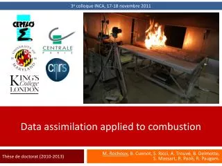
3 e colloque INCA, 17-18 novembre 2011. Data assimilation applied to combustion. M. Rochoux , B. Cuenot, S. Ricci, A. Trouvé, B. Delmotte, S. Massart, R. Paoli, R. Paugam . Thèse de doctorat (2010-2013). Data assimilation. Physical system. ↘ MEASUREMENTS. ↘ NUMERICAL MODEL.

E N D
3e colloque INCA, 17-18 novembre 2011 Data assimilation applied to combustion M. Rochoux, B. Cuenot, S. Ricci, A. Trouvé, B. Delmotte, S. Massart, R. Paoli, R. Paugam. Thèse de doctorat (2010-2013)
Data assimilation Physical system ↘ MEASUREMENTS ↘ NUMERICAL MODEL • Control variables • Uncertainty quantification • Observable quantity • Uncertainty quantification ↘ PRINCIPLE Integrate observations into a running model in such way as to minimize the error, using known error statistics on both simulated and observed data.
Data assimilation Physical system ↘ MEASUREMENTS ↘ NUMERICAL MODEL • Control variables • Uncertainty quantification • Observable quantity • Uncertainty quantification ↘ BENEFITS • Compare experiment and simulation. • Quantify and reduce uncertainties. • Optimize an observation network.
Application to combustion • Sources of uncertainties in CFD • Simplification of the physics • ↘ Ex.: Turbulent flame speed, burner extinction. • Physical and numerical parameters. • Boundary conditions • ↘ Ex.: Heat transfer to the walls, spray injection. • Initial condition • ↘ Ex.: Burner ignition. Potential of data assimilation • Improve simulations via improved initial/boundary condition. • Improve physical models via calibrated parameters. • Optimize place and time of probe measurements.
Research framework Data assimilation for wildfire spread Towards a more accurate prediction of flame propagation. • Bénédicte Cuenot • Sophie Ricci • Denis Veynante • Nasser Darabiha • Arnaud Trouvé • Today’s outline • ↘ Data-driven model parameter estimation for flame propagation. • Description of the physical system. • Data assimilation algorithm. • Validation on a synthetical case. • Application to a real case of fire propagation.
1. Description of the physical system Model of flame propagation FRESH AREA • Objective • ↘Build a simplified model of premixed flame that gives the time-evolution of the flame front. • Scalar progress variable c • ↘ Interface between burnt and fresh fuel (c = 0.5). • ↘ Front propagating at the local flame speed ϒ. FRONT BURNT AREA c = 1 BURNT AREA 2-D computational domain Level-Set equation ϒ c = 0.5 FRONT FRESH AREA Local flame speed ↘Parameterization in terms of a reduced number of parameters. ↘Linked to fuel mixture and flow conditions. c = 0
1. Description of the physical system Model of flame propagation FRESH AREA • Objective • ↘Build a simplified model of premixed flame that gives the time-evolution of the flame front. • Scalar progress variable c • ↘ Interface between burnt and fresh fuel (c = 0.5). • ↘ Front propagating at the local flame speed ϒ. FRONT BURNT AREA c = 1 BURNT AREA 2-D computational domain Level-Set equation ϒ c = 0.5 FRONT FRESH AREA Local flame speed c = 0 Proportionality coefficient (m/s) Random field of fuel mass fraction
1. Description of the physical system Simulation vs. Experiments • Example of fire spread simulation • ↘Constant coefficient: P = 0.1 m/s. • ↘ Size of computational domain: 300m x 300m. • ↘ Initial condition: semi-circular front. Input data ↘ Random fuel mass fraction Simulation outputs ↘ Time-evolving location of the flame front (from t=0 to t=800s) Observation at t=800s • How to compare quantitatively simulation and experiments? • How to make simulations more reliable? Data assimilation for parameter calibration
2. Data assimilation algorithm Variables of interest • STEP. 1: Description of the physical system • Observation vector yo • ↘ 2-D coordinates of the points defining the observed fronts. • ↘ Several observed fronts over the assimilation time window [0,T].
2. Data assimilation algorithm Variables of interest • STEP. 1: Description of the physical system • Observation error covariance matrix R • ↘ Observation error following a Gaussian distribution N(0,R). • ↘ Uncorrelated errors in space and time: diagonal matrix R.
2. Data assimilation algorithm Variables of interest • STEP. 1: Description of the physical system • Control vector x • ↘ Contains the control parameters that are to be optimized. • ↘ Estimate of the true value xt, starting from an a priori value xb. Background
2. Data assimilation algorithm Variables of interest • STEP. 1: Description of the physical system • Background error covariance matrix B • ↘ Background error following a Gaussian distribution N(0,B). • ↘ Diagonal elements > Error variance on each control parameter.
2. Data assimilation algorithm Variables of interest • STEP. 2: Definition of the observation operator H • Non-linear operator, resulting from a 2-step operation: • ↘ Model integration over the assimilation time window. • ↘ Selection operator (from field c to front isocontour c=0.5).
2. Data assimilation algorithm Variables of interest • STEP. 3: Distance between simulated and observed fronts • Formulation of the innovation vector dob • ↘ At each observation time, projection of the simulated front • onto the observed front.
2. Data assimilation algorithm Variables of interest • STEP. 4: Gain matrix K • Weight of the data assimilation correction. • Requires the Jacobian of the observation operator H • ↘ Not available analytically. • ↘ Jacobian matrix called the tangent linear H. here,
2. Data assimilation algorithm Variables of interest • STEP. 5: Analysis xa • Feedback information for the model (inverse problem). • Optimal estimation of the true control vector xt, such that the variance of its distance to xt gets a minimum.
2. Data assimilation algorithm Best Linear Unbiased Estimator (BLUE) • Kalman filter approach • ↘ Analysis xaas the correction of the background vector xb • ↘ Assumption of a linear observation operator H. Analysis error covariance matrix • Adaptation of the BLUE algorithm: iterative process
2. Data assimilation algorithm Best Linear Unbiased Estimator (BLUE) • Kalman filter approach • ↘ Analysis xaas the correction of the background vector xb • ↘ Assumption of a linear observation operator H. Analysis error covariance matrix Reduction of the variance • In the observation space Validation criteria Reduction of the variance of the distance between fronts.
3. Validation Synthetical case of flame propagation • Observation System Simulation Experiment (OSSE) • ↘ Knowntrue control vector, background and observation errors. • ↘Generation of synthetical observations using the numerical model • Integrate numerical model using the true control vector. • Add noise to the fronts positions. • Quantify the quality of the background correction. • Validate the data assimilation algorithm.
3. Validation Synthetical case of flame propagation • Validation experiment for one parameter calibration • ↘ True control vector: xt = Pt = 0.1 • ↘ Fixed observation standard deviation: σo = 0.0073m. • Observed front discretized with 200 points. • 16 observation times each 50s. • ↘ Assimilation time window [0,800s]. • ↘ Background xb varying from 0.02 to 0.18 Error standard deviation on the analysis xa systematically reduced SCENARIO: High confidence in the observation. VARIABLE background standard deviation σb Analysis xa equal to xt with less than 0.1% (very low number of external loops - 2 or 3). RESULTS From 20% to 80% True value From -20% to -80%
4. Application to a real case Natural fire propagation • Real observations of flame positions • ↘ Domain of propagation: 4m x 4m • ↘ Homogeneous grass vegetation • Height: 8cm • Fuel loading: 0.4 kg/m2 • Moisture content: 21.7% Ignition times From 0 to 0.02m/s Rate of spread Wind (1.3 m/s) Data from Ronan Paugam, Dept. Of Geography, King’sCollege of London
4. Application to a real case Natural fire propagation • Model for the fire rate of spread • ↘ New parameterization of the flame speed • vegetation characteristics (moisture content Mf, surface-area-to-volume ratio Σ). • wind velocity along the normal direction to the front u. Rothermel’s model
4. Application to a real case Natural fire propagation • Calibration of 2 vegetal parameters • ↘ Parameters that are critical for the rate of spread and that are embedded with important uncertainties. • Moisture content. • Surface-area-to-volume ratio. Reduction of the variance on the control parameters. • ↘ Assimilation time window [51s,78s] • 1 observation time at t=78s. • observation error: linked to spatial resolution 0.047m. • background error: 30% uncertainty. RESULTS • Control parameters still in their domain of validity. • Σ far from typical value. • over-correction to compensate for the uncertainties in the rate of spread Γ.
4. Application to a real case Natural fire propagation • Assimilation & Forecast • ↘ Assimilation time window [51s,78s]
4. Application to a real case Natural fire propagation • Assimilation & Forecast • ↘ Assimilation time window [51s,78s] • ↘ Forecast time window [78s,106s] ANALYSIS t = 78s FORECAST t = 106s
Conclusion • Data assimilation for flame propagation • Algorithm able to retrieve more accurate value of the control parameters • ↘ Turbulent flame speed, burner extinction. • Physical and numerical parameters. • Boundary conditions • ↘ Ex.: Heat transfer to the walls, spray injection. • Initial condition • ↘ Ex.: Burner ignition. Résultats ↘ Gain significatif d’informations sur le système en prenant en compte les observations. ↘ Réduction et estimation de l’incertitude sur le résultat de l’assimilation de données. ↘ Prédiction de l’évolution du système comme en météorologie. Perspectives ↘ Utilisation de l’assimilation de données comme un outil d’aide à la modélisation de la propagation des feux. ↘ Extension possible à d’autres problématiques en combustion.