Genetic Programming
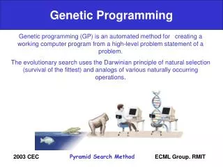
Genetic Programming (GP), developed by J. Koza in the 1990s in the USA, is a type of evolutionary algorithm primarily used for machine learning tasks such as prediction and classification. GP applies unique features including non-linear chromosomes (trees, graphs) and requires large populations for optimal performance. It faces competition from neural networks yet can be particularly effective in tasks like credit scoring. GP utilizes tree-based representations for constructing solutions, enabling the exploration of a vast search space for optimal formula identification.

Genetic Programming
E N D
Presentation Transcript
GP quick overview • Developed: USA in the 1990’s • Early names: J. Koza • Typically applied to: • machine learning tasks (prediction, classification…) • Attributed features: • competes with neural nets and alike • needs huge populations (thousands) • slow • Special: • non-linear chromosomes: trees, graphs • mutation possible but not necessary (disputed!)
Introductory example: credit scoring • Bank wants to distinguish good from bad loan applicants • Model needed that matches historical data
Introductory example: credit scoring • A possible model: IF (NOC = 2) AND (S > 80000) THEN good ELSE bad • In general: IF formula THEN good ELSE bad • Only unknown is the right formula, hence • Our search space (phenotypes) is the set of formulas • Natural fitness of a formula: percentage of well classified cases of the model it stands for • Natural representation of formulas (genotypes) is: parse trees
AND = > NOC 2 S 80000 Introductory example: credit scoring IF (NOC = 2) AND (S > 80000) THEN good ELSE bad can be represented by the following tree
Tree based representation • Trees are a universal form, e.g. consider • Arithmetic formula • Logical formula • Program (x true) (( x y ) (z (x y))) i =1; while (i < 20) { i = i +1 }
Tree based representation i =1; while (i < 20) { i = i +1 }
Tree based representation • In GA, ES, EP chromosomes are linear structures (bit strings, integer string, real-valued vectors, permutations) • Tree shaped chromosomes are non-linear structures • In GA, ES, EP the size of the chromosomes is fixed • Trees in GP may vary in depth and width
Tree based representation • Symbolic expressions can be defined by • Terminal set T • Function set F (with the arities of function symbols) • Adopting the following general recursive definition: • Every t T is a correct expression • f(e1, …, en) is a correct expression if f F, arity(f)=n and e1, …, en are correct expressions • There are no other forms of correct expressions
GA flowchart GP flowchart
Mutation • Most common mutation: replace randomly chosen subtree by randomly generated tree
Mutation cont’d • Mutation has two parameters: • Probability pm to choose mutation vs. recombination • Probability to chose an internal point as the root of the subtree to be replaced • Remarkably pm is advised to be 0 (Koza’92) or very small, like 0.05 (Banzhaf et al. ’98) • The size of the child can exceed the size of the parent
Recombination • Most common recombination: exchange two randomly chosen subtrees among the parents • Recombination has two parameters: • Probability pc to choose recombination vs. mutation • Probability to chose an internal point within each parent as crossover point • The size of offspring can exceed that of the parents
Parent 1 Parent 2 Child 1 Child 2
Selection • Parent selection typically fitness proportionate • Over-selection in very large populations • rank population by fitness and divide it into two groups: • group 1: best x% of population, group 2 other (100-x)% • 80% of selection operations chooses from group 1, 20% from group 2 • for pop. size = 1000, 2000, 4000, 8000 x = 32%, 16%, 8%, 4% • motivation: to increase efficiency, %’s come from rule of thumb • Survivor selection: • Typical: generational scheme (thus none) • Recently steady-state is becoming popular for its elitism
Initialisation • Maximum initial depth of trees Dmax is set • Full method (each branch has depth = Dmax): • nodes at depth d < Dmax randomly chosen from function set F • nodes at depth d = Dmax randomly chosen from terminal set T • Grow method (each branch has depth Dmax): • nodes at depth d < Dmax randomly chosen from F T • nodes at depth d = Dmax randomly chosen from T • Common GP initialisation: ramped half-and-half, where grow & full method each deliver half of initial population
Bloat • Bloat = “survival of the fattest”, i.e., the tree sizes in the population are increasing over time • Ongoing research and debate about the reasons • Needs countermeasures, e.g. • Prohibiting variation operators that would deliver “too big” children • Parsimony pressure: penalty for being oversized
Problems involving “physical” environments • Trees for data fitting vs. trees (programs) that are “really” executable • Execution can change the environment the calculation of fitness • Example: robot controller • Fitness calculations mostly by simulation, ranging from expensive to extremely expensive (in time) • But evolved controllers are often to very good
Example application: symbolic regression • Given some points in R2, (x1, y1), … , (xn, yn) • Find function f(x) s.t. i = 1, …, n : f(xi) = yi • Possible GP solution: • Representation by F = {+, -, /, sin, cos}, T = R {x} • Fitness is the error • All operators standard • pop.size = 1000, ramped half-half initialisation • Termination: n “hits” or 50000 fitness evaluations reached (where “hit” is if | f(xi) – yi | < 0.0001)
Discussion Is GP: The art of evolving computer programs ? Means to automated programming of computers? GA with another representation?
Introduction to GP based identification Model System Model structure Model parameters Black-box models Model-selection Known parameters Based on prior knowledge Black-box modeling A modellező választmodell struktúrát Identification From measured datawith some optimization
Linear in parameters model The original GP generates models that are nonlinear in their parameters Linear in parameters model The parameters can be estimated by LS
Model representation + + * x3 x1 + * F2 x1 x1 x2 x2 F3 F1
OLS • With orthogonal LS we can estimate the contribution • The useless branches will be deleted + + + * x1 * x3 x1 + * F1 x1 x2 F2 F2 x1 x1 x2 x2 F3 F1
4 3 2 1 0 -1 -2 0 20 40 60 80 100 (y) + 4% noise (u) Example: system-identification simulation Result of GP
Improvement of the OLS 10-10 runs with max. 1000 evaluations • : No penaly on the size of the tree • : Penaly on the size of the tree • : penaly on the size of the tree + OLS
Conclusions • Model structure identification is a not trivial task • GP can be used for this purpose • Linear in parameters models are ideal for GP based structure exploration • It is useful to apply OLS to regularize the tree

