Comparing Small Independent and Dependent Samples in Sociology Research
230 likes | 346 Vues
This document explores the methodology for comparing small sample means and proportions between independent and dependent groups in sociology. It details the differences between two small sample means, highlighting the implications of using dependent samples, also known as matched pairs or paired difference data. The significance tests for dependent means, particularly McNemar's test for dependent proportions, are examined using a specific example involving undergraduate students' geography test scores across two time points (2001 and 2002). Understanding these comparisons is vital for accurate research analysis.

Comparing Small Independent and Dependent Samples in Sociology Research
E N D
Presentation Transcript
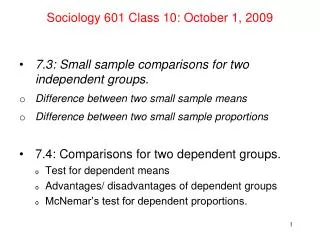
Sociology 601 Class 10: October 1, 2009 • 7.3: Small sample comparisons for two independent groups. • Difference between two small sample means • Difference between two small sample proportions • 7.4: Comparisons for two dependent groups. • Test for dependent means • Advantages/ disadvantages of dependent groups • McNemar’s test for dependent proportions.
7.4 Dependent samples • Dependent samples occur when each observation in the first sample has something in common with one observation in the second sample. • Also called matched pairs data. • Also called paired difference data. • Also called a randomized block design. • Repeated measurement data fall into this category. • In a data set, dependent samples often appear as two variables for each respondent in the data set.
Dependent samples: an example • Suppose that a researcher in geography had surveyed a small sample of undergraduates in May 2001, and collected answers to a series of questions on world geography. • In May 2002, that researcher decided to retest the students to see if knowledge of world geography increased after the events of 9/11/2001
Data set for geography example. • Scores for May 2001 sample: • (5,2,8,3,6,4,7) (n=7, Ybar1 = 5, s.d. = 2.16) • Scores for May 2002 sample: • (6,4,9,_,10,5,8) (n=6, Ybar2 = 7, s.d. = 2.37) • Each score in 2001 matches the corresponding score in 2002. • The fourth student, who scored a 3 in 2001, refused to participate in May 2002.
A comparison for dependent samples Enter the scores as separate variables, matched by respondent clear input id scor2001 scor2002 1 5 6 2 2 4 3 8 9 4 3 . 5 6 10 6 4 5 7 7 8 end
A comparison for dependent samples The t-test for dependent samples would look like this: . ttest scor2001=scor2002 Paired t test ------------------------------------------------------------------------------ Variable | Obs Mean Std. Err. Std. Dev. [95% Conf. Interval] ---------+-------------------------------------------------------------------- scor2001 | 6 5.333333 .8819171 2.160247 3.066293 7.600373 scor2002 | 6 7 .9660918 2.366432 4.516582 9.483418 ---------+-------------------------------------------------------------------- diff | 6 -1.666667 .4944132 1.21106 -2.937596 -.395737 ------------------------------------------------------------------------------ Ho: mean(scor2001 - scor2002) = mean(diff) = 0 Ha: mean(diff) < 0 Ha: mean(diff) != 0 Ha: mean(diff) > 0 t = -3.3710 t = -3.3710 t = -3.3710 P < t = 0.0099 P > |t| = 0.0199 P > t = 0.9901
Significance test for paired differences • We give a random sample of seven UM students a set of world geography questions in May 2001, then in May 2002. We obtain matched scores for six of the students. • Dbar = 1.67, s.d. = 1.211, n = 6 • Decide whether test scores were different in 2002 than in 2001.
Significance test for paired differences • Assumptions: • We are working with a random sample of UM students. • The difference is measured as an interval-scale variable • Difference scores are normally distributed in the population, or the number of pairs is 30 or more. • Hypothesis: • There is no average difference between a student’s score in 2002 and the student’s score in 2001. • Ho: D = 0
Significance test with dependent samples • Test statistic: • The test statistic for D (for n matched pairs) is… • t = Dbar/ (sD/ sqrt(n)) = 1.67 / (1.211/√6) = 3.371 • d.f. = n – 1 = 6 – 1 = 5
Significance test with dependent samples • t = 3.371, d.f.= 5 • P-value: • move down the columns to df = 5 • move across to the t-scores that bracket 3.371: • for column 4, t = 3.365. for column 5, t=4.032 • move up to read the one-sided p-values • .01 > p > .005 one-sided. • double the p-value to translate to a 2-sided p-value • .02 > p > .01 two sided, so p < .02
Significance test with dependent samples • p < .02 two-sided. • Conclusion: • It is very unlikely that the difference in scores could have occurred by chance alone, so we reject the null hypothesis and conclude that the geography scores were different (increased) from 2001 to 2002. • It is difficult to judge the substantive importance of the difference without knowing more about the test. The average difference was somewhat smaller than the typical variation among students.
Confidence interval for dependent samples: • The confidence interval for D is… • (Essentially, statistical inference for the difference between dependent samples is the same as statistical inference for a single sample mean.)
Advantages and disadvantagesof a matched sample test • Known sources of potential bias are controlled. For example, comparing students who had taken the course with students who had not would probably be biased since the course probably selects out students already interested in (and so know more about) geography. (+) • The standard deviation of the test statistic is usually smaller, making the power of your test proportionately greater. (+) • Matched tests can be relatively expensive to do, because you have to find the same subjects, and you might lose some to attrition. (-) • If you reject the null hypothesis, you may have difficulty arguing that the difference is due to global events instead of a test-retest “practice effect”. (-)
Dependent versus independent samples When is it appropriate to use a dependent-samples design? • repeated measures for the same individual/ area/ class? YES • studies with matched pairs of family members? YES • studies with samples matched for levels of another variable? YES (but multivariate statistics are better) • studies matched by values of the outcome under study? NO, that would be cheating. • studies matched at random, say by caseid for separate samples? NO, not acceptable by convention. (On average this would provide no help, but if you do it as a fishing expedition, you might randomly soak up a bit of the unexplained error.)
Using “error” to understand the difference between independent and dependent samples. • Think of an observed score as a sum of the population mean and “error” for that case. Yi = μ + ei • ei includes any factors that cause the score to differ from the mean: • individual differences • differences unique to the observation • measurement error • Across the population, error has an average of 0 and a typical value of ± σ
Error in a difference between scores • The difference between two scores can be describes thusly: Y2i- Y1i= (μ2 + e2i) – (μ1 + e1i) = (μ2 - μ1) + (e2i - e1i) where (μ2 - μ1) is the population difference we’re interested in and where (e2i - e1i) is the unwanted variation • If e2i is independent of e1i, then (e2i - e1i) will be larger than either error alone by a factor of √2 (on average) • However, if e2i and e1i have a shared error component, then (e2i - e1i) will subtract out the shared error, thereby making it easier to study (μ2 - μ1)
Error in a difference between scores In the example of pairs of geography test scores, define the following as “shared error”, “unshared error”, or something else. • Some of the respondents have a strong prior geography background. • One of the respondents was feeling sick the day of the 2002 test. • One respondent guessed at all the answers both times. • Three of the respondents read some books about the Middle East and South Asia between 2001 and 2002. • In 2002, two of the respondents vaguely remembered the test questions from the previous year.
Comparing proportions in dependent samples: • A survey asked 340 registered voters their opinions about government spending. • 90% (306 favored more spending on law enforcement. • 93.24% (317) favored more spending on health care. • You can break this pattern down further • 292 favored more spending for both • 9 favored less spending for both • 25 favored more for health, less for law • 14 favored more for law, less for health
Comparing proportions in dependent samples • Assumptions: • The observations were drawn as a random sample. • We are working with categorical data • We need to assume minimum sample size for a normal sampling distribution: n12 + n21 > 20 • Hypothesis: • There is no difference in the proportion supporting either social program • H0: πlaw – πhealth = 0
Comparing proportions in dependent samples • Test statistic: • The test statistic for a comparison of paired proportions is a z-score, estimated using McNemar’s Test. • z = (n12 - n21) / √(n12 + n21) • Z = (25 – 14) / √(25+14) = 11/6.245 = 1.76
Comparing proportions in dependent samples • P-value: for z=1.76, p=.08 (two-tailed) • Conclusion: I would not reject the null hypothesis. In the sample it appears that increased health spending may be more popular than increased spending on law enforcement, but this difference could have occurred by chance alone.
How is McNemar’s test derived? • P1 = (n11+ n21)/ ntotalP2 = (n11+ n12) / ntotal • Difference of population proportions: P1 – P2 = (1*n12 +(-1)* n21 +0*n11 +0*n22 ) / ntotal = (n12 - n21) / ntotal • Standard error of difference (the tough one): s.e. = SQRT (P1(1-P1)+ P2(1-P2) - 2 (P11*P22 - P12*P21) / n) = SQRT((n12 + n21)) / ntotal • Z-score: z = (P1 – P2) / s.e. = (n12 - n21) / SQRT((n12 + n21))
An alternative to McNemar’s Test in STATA. • The TTEST command can also be used for comparing dependent samples when the samples are proportions. • Assume you have downloaded a data set with case-by-case data for variables “health” and “law” . ttest health=law Paired t test ------------------------------------------------------------------------------ Variable | Obs Mean Std. Err. Std. Dev. [95% Conf. Interval] ---------+-------------------------------------------------------------------- health | 340 .9323529 .01364 .2515094 .9055232 .9591827 law | 340 .9 .0162938 .3004422 .8679504 .9320496 ---------+-------------------------------------------------------------------- diff | 340 .0323529 .0183106 .3376306 -.0036637 .0683696 ------------------------------------------------------------------------------ Ho: mean(health - law) = mean(diff) = 0 Ha: mean(diff) < 0 Ha: mean(diff) ~= 0 Ha: mean(diff) > 0 t = 1.7669 t = 1.7669 t = 1.7669 P < t = 0.9609 P > |t| = 0.0781 P > t = 0.0391