Download
1 / 108
1.09k likes | 1.24k Vues
4 COORDINATED REPLENISHMENTS cyclic schedules powers-of-two policies. 4.1 Powers-of-two policies Cycle times are restricted to be powers of two times a certain basic period denoted as q . From (3.5) in Chapter 3, we have:. , (4.1) Let T = Q/d, T * = Q * /d .

E N D
4 COORDINATED REPLENISHMENTS • cyclic schedules • powers-of-two policies
4.1 Powers-of-two policies Cycle times are restricted to be powers of two times a certain basic period denoted as q . From (3.5) in Chapter 3, we have: , (4.1) Let T = Q/d, T* = Q*/d . (4.2)
Lot sizing problem (4.3) Worst scenario: Because the cost is convex, the worst possible error must occur when two consecutive values of m, say m = k and m = k + 1 give the same error. Let T < T* correspond to m = k, and 2T > T* to m = k + 1. . (4.4)
C/C* T T2 T T1 T* 2T2 2T 2T1 , (4.5) . (4.6) Proposition 4.1 For a given basic period q, the maximum relative cost increase of a powers-of-two policy is 6 percent.
Note that T1 gives better cost than Note that 2T2 gives better cost than
Suppose possible to change q For a single item, the optimal solution is to choose q equal to a power of two times T*. For N items, we can, in general, not fit q perfectly to all cycle times Ti*. The relative cost increase can be expressed as:
. (4.7) We know from (4.2) and (4.5) that for a given q, each can be expressed as : (4.8) The weights wi for the different values of xi , can be seen as a probability distribution F(x) on [-1/2, 1/2], i.e., F(-1/2) = 0 and F(1/2) = 1.
. (4.9) Change q by multiplying by 2y , This means that a certain x is replaced by x + y for x + y≤ ½, , and by x + y - 1 for x + y > ½.
(4.10) For a given distribution F(x) the minimum cost increase is obtained by minimizing (4.10) with respect to 0 ≤ y≤ 1.
Proposition 4.2 If we can change the basic period q, the maximum relative cost increase of a powers-of-two policy is 2 percent. Proof The average cost increase for 0 ≤ y≤ 1 must be at least as large as the minimum
The worst case will occur when the distribution F(x) is uniform on , see (4.9). A change of q will then not make any difference.
u 1 1/2 y 0 1 1 = - u y 2 1 = + y u -1/2 2 Given y Given u
u 1 1/2 0 y -1/2 Given y Given u
4.2 Production smoothing Mixed integer program (MIP) Manne (1958) Billington et al. (1983) Eppen and Martin (1987) Shapiro (1993) Objective: Low inventory cost and smooth capacity utilization. Simplification: ignore stochastic variations ignore time-varying aspect MIP not used in practice
When the demands for different items are relatively stable, use cyclic schedules. In a general case with many items and several production facilities, it can be extremely difficult to find suitable cyclic schedules. It is also common in practice to smooth production outside the inventory control system. Each item ordered periodically. Ordering period chosen to smoothen the load.
Example: 4 items, same demand Item 1: 1,5,9 Item 2: 2,6,10 Item 3: 3,7,11 Item 4: 4,8,12 Periodic review: order up to S policy Continuous review: large variation in production load resulting in long and uncertain lead time.
4.2.1 The Economic Lot Scheduling Problem (ELSP) Cyclic schedules for a number of items with constant demands. Backorders not allowed. Finite production rate Single production facility
Notation: N = number of items, hi = holding cost per unit and time unit for item i, Ai = ordering or setup cost for item i, di = demand per time unit, pi = production rate (pi > di), si = setup time in the production facility for item i, independent of the sequence of the items, Ti = cycle time for item i (the batch quantity Qi = Tidi).
Define: i = di/pi , i = iTi = production time per batch for item i excluding setup time, i = si+ i= total production time per batch for item i.
Table 4.1 N = 10 Bomberger (1966) Table 4.1 Bomberger’s problem (time unit = one day). . (4.11) The problem is to minimize subject to the constraint that all items should be produced in the common production facility.
The optimal cycle time when disregarding the capacity constraint is , (4.12) . (4.13) Note that (4.11) and (4.12) are equivalent to (3.6) and (3.7) if we replace Ti by Qi/di , and i by di/pi .
Table 4.2 Independent solution of Bomberger’s problem. , is a lower bound for the total costs.
9.30 Item 9 Item 9 • Solution not feasible: Consider items 4, 8 and 9. Item 4 & 8 have cycle times 19.5 and 20.5. Must be able to produce one batch of #4 and #8 in [t,t+20.5], or [t+11.20,t+20.5]. But the length of available time is 9.30, while 4+8 =10.16 >9.30. Not feasible 11.20 t t+20.5 t+61.5
Does a feasible solution exist? If at least one setup time is positive an obvious necessary condition for a feasible solution to exist is . (4.14) Condition (4.14) is also sufficient for feasibility. Given the assumption of a common cycle time, the problem now is to minimize , (4.15)
with respect to the constraint that the common cycle must be able to accommodate production lots of all items . (4.16) , (4.17) a lower bound for the cycle time. Need large enough T to squeeze setups in the slack 1-
Disregard (4.17), from (4.15) . (4.18) Since (4.15) is convex in T the optimal solution, , (4.19) For Bomberger’s problem, Tmin = 31.86, and consequently, . cost=41.17. For problems where the individual cycle times are reasonably similar, the common cycle approach gives a very good approximation.
Two approaches for deriving better • solutions. • Dynamic programming model • Bomberger (1966) • Assuming • Ti = niW • W should be able to accommodate production of • all items.
Fi(w) = minimum cost of producing items i +1,i+2,..., N when the vailable capacity in the basic period is w, i.e., W - w has been used for items 1, 2,...,i. , (4.20) where Ci(niW) are the costs (4.11) for item i with Ti = niW, si = si + riniW, and the integer ni is subject to the constraint . (4.21) or Note that the upper bound in (4.21) is equivalent to si w. FN(w) = 0 for all w 0. F0(W) gives the minimum costs when the basic period is equal to W.
Minimize over W. Bomberger’s solution C=36.65, W=40, ni=1 for i 7, n7 =3. • Serious Assumption: W should be able to accommodate production of all items.
II. Heuristic • Doll and Whybark, 1973). • The procedure is to successively improve the multipliers niand the basic period W according to the following iterative procedure: • Determine the independent solution and use the • shortest cycle time as the initial basic period W. • 2. Given W, choose powers-of-two multipliers, • (ni = 2mi, mi 0), to minimize the item costs (4.11).
3. Given the multipliers ni , minimize the total costs with respect to W. 4. Go back to Step 2 unless the procedure has converged. In that case, check whether the obtained solution is feasible. If the solution is infeasible, try to adjust the multipliers and then go back to Step 3. Compare with independent solution.
Apply the heuristic to Bomberger’s problem. Table 4.3 Solution of Bomberger’s problem with W = 23.42.
In case of stochastic demand, one possible approach is to first solve a deterministic problem based on averages, and then try to adapt the solution to the stochastic case by adding suitable safety stocks.
4.2.2 Production smoothing and batch quantities Adjust the batch quantities to obtain a reasonably smooth load. Karmarkar (1987, 1993). Axsäter (1980, 1986), Bertrand (1985), and Zipkin (1986).
Consider a machine in a large multi-center shop. D = average output of material (demand), units per time unit, P = average processing rate, units per time unit, Q = batch quantity, t = setup time, T = average time in the system for a batch, h = holding cost per unit and time unit after processing.
Assume: The batches arrive at the machine as a Poisson process with rate l = D/Q. Thus Av demand=Q=D. The processing time is exponentially distributed. average processing time for a batch is 1/k = t + Q/P. Service rate =. = l / = Dt/Q + D/P. The average time spent in the M/M/1 system is . (4.22) The average cycle stock is approximated as Q/2.
Assume that the average holding cost per unit and time unit for work-in-process is exactly half of the holding cost h after the process. Av cycle stock = Q/2. Total holding cost after the process=hQ/2. Work-in-process TD=Av time in the system * Av demand .(4.23) . (4.24) For low values of D, Q* is essentially linear in D. For larger values, Q* grows very rapidly.
4.3 Joint replenishments 4.3.1 A deterministic model Setup costs: Individual setup costs for each item, and a joint setup cost for the whole group of items. Reason: joint setup costs, quantity discounts, coordinated transports. constant continuous demand. No backorders. batch quantities are constant. production time is disregarded. No lead time or the lead time is same for all items.
Notation: N = number of items, hi = holding cost per unit and time unit for item i, A = setup cost for the group, ai = setup cost for item i, di = demand per time unit for item i, Ti = cycle time for item i. i= hidi Assume all demands equal to one. Items are ordered so that a1/1 a2/ 2 ... aN/N . Note that increasing setup costs and decreasing holding costs mean increasing lot sizes and cycle times.
Approach 1. An iterative technique If there were no joint setup cost , (4.25) i.e., T1 would be the smallest cycle time. Assume other cycle times of items 2, 3... N are integer multiples ni of the cycle time for item 1, , i = 2, 3,..., N. (4.26) Our objective is to minimize w.r.t T1, n2, n3, ... nN the cost. ,(4.27) Fix cost ith item holding cost=Tinii/2
Given n2, n3... nN, , (4.28) . (4.29) Note that T1 is not chosen according to (4.25).If we disregard n2, n3... nN to be integers, then from (4.29), . (4.30) From (4.30) and (4.29), the lower bound for the costs: .(4.31)
HEURISTIC • Determine start values of n2, n3... nN by rounding • (4.30) to the closest positive integers. • 2. Determine the corresponding T1 from (4.28). • 3. Given T1, minimize (4.27) with respect to n2, n3... nN. • This means that we are choosing ni as the positive • integer satisfying . (4.32) Return to Step 2, if any multiplier ni has changed since the last iteration.
Example 4.1 N = 4 , A = 300, a1 = a2 = a3 = a4 = 50, h1 = h2 = h3 = h4 = 10, d1 = 5000, d2 = 1000, d3 = 700, and d4 = 100. As requested, ai/hi is nondecreasing with i. When applying the heuristic we obtain again n2 = 1, n3 = 1, n4 = 3, i.e., the algorithm has already converged.
Approach 2. Roundy´s 98 percent approximation the joint setups have cycle time T0 0, , i = 1, 2, ..., N, (4.33) where ki is a nonnegative integer. Let a0 = A, and h0 = 0, , (4.34) subject to the constraints (4.33). replacing (4.33) by , i = 1, 2, ..., N. (4.35)
The resulting solution will give a lower bound for the costs.I lagrangian relaxation , (4.36) where li are nonnegative. define = h1 - 2l1, . . (4.37) . =hN - 2lN.
the optimal solution must have allThe optimal solution of the relaxed problem can be obtained by solving N + 1 independent classical lot sizing problems. (4.38) without any constraints on the cycle times. rounding the cycle times of the relaxed problem, (4.39)
for some number q > 0. From Proposition 4.1, if q is given, the maximum cost increase is at most 6 percent. If we adjust q to get a better approximation the cost increase is at most 2 percent according to Proposition 4.2. We have now obtained Roundy’s solution of the problem.