Download
1 / 35
410 likes | 850 Vues
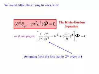
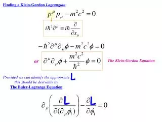
Finding a Klein-Gordon Lagrangian. or. The Klein-Gordon Equation. L. Provided we can identify the appropriate this should be derivable by The Euler-Lagrange Equation. L. L. I claim the expression . L. serves this purpose. L. L. L. L. L. L. L. L.

E N D
Finding a Klein-Gordon Lagrangian or The Klein-Gordon Equation L Provided we can identify the appropriate this should be derivable by The Euler-Lagrange Equation L L
I claim the expression L serves this purpose
L L L L L L L L
You can (and will for homework!) show the Dirac Equation can be derived from: LDIRAC(r,t) We might expect a realistic Lagrangian that involves systems of particles L(r,t) = LK-G + LDIRAC but each term describes free non-interacting particles describes photons describes e+e-objects L + LINT But what does terms look like? How do we introduce the interactions the experience?
We’ll follow (Jackson) E&M’s lead: A charge interacts with a field through: current-field interactions the fermion (electron) the boson (photon) field from the Dirac expression for J particle state antiparticle (hermitian conjugate) state Recall the “state functions” have coefficients that must satisfy anticommutation relations. They must involve operators! What does such a PRODUCT of states mean?
We introduce operators (p) and †(p) satisfying either of 2 cases: or Along with a representation of the (empty) vacuum state: | 0 such that:
The Creation Operator It's alive! ALIVE! † X (p) † X (p) | 0 > = | p >
“creates” a free particle of 4-momentum p The complex conjugate of this equation reads: The above expression also tells us: |0 which we interpret as:
THE ANNIHILATOR The Annihilation Operator X (p) X (p) | p > = 0
If we demand, in general, the orthonormal states we’ve assumed: 1 0 0 0 0 an operation that makes no contribution to any calculation
Then [ (p-q) †(p)(q) ] |0 †(p)|0 = zero =(p-q)|0 This is how the annihilation operator works: If a state contains a particle with momentum q, it destroys it. The term simply vanishes (makes no contribution to any calculation) if p q. |p1 p2 p3=†(p1)†(p2)†(p3) |0
or in contrast †(p)†(k)|0 =†(k)†(p)|0 †(p)†(k)|0 =-†(p)†(k)|0 |pk =|kp |pk =-|kp |pp =|pp 0 and if p=k this must give and if p=k this gives This is perfectly OK! These must be symmetric states These are anti-symmetric states BOSONS FERMONS
Recall the most general DIRAC solution: s s dk3 k g h s that these Dirac particles are fermions {(r,t),†(r´,t)} =d 3(r – r) If we insist: we can identify (your homework) g as an annihilation operator a(p,s) and h as a creation operator b†(-p,-s) a b† † a b
Similarly for the photon field (vector potential) [A(r,t),A†(r´,t)] =d 3(r – r) If we insist: Bosons! † -s -k -s -k d d Remember here there is no separate anti-particle (but 1 particle with 2 helicities). Still, both solutions are needed for mathematical completeness.
Now, since interactions between Dirac particles (like electrons) and photons appear in the Lagrangian as It means these interactions involve operator products of (a†+b) (a+b† ) (d† +d) creates an electron annihilates an electron creates a photon annihilates a photon annihilates a positron creates a positron giving terms with all these possible combinations: a†b†d† a†ad† a†ad† a†ad bb†d† bb†d bad† bad
What do these mean? a†b†d† a†ad† a†ad† a†ad bb†d† bb†d bad† bad In all computations/calculations we’re interested in, we look for amplitudes/matrix elements like: 0|daa†|0 Dressed up by the full integrals to calculate the probability coefficients creates a positron e+ e- e- a†b†d† a†ad† e- creates an electron creates a photon annihilates an electron
e- a†ad† time e- e- a†ad time e-
Particle Physicists Awarded the Nobel Prize since 1948 1948 Lord Patrick Maynard Stuart Blackett For development of the Wilson cloud chamber 1949 Hideki Yukawa Prediction of the existence of mesons as the mediators of nuclear force 1950 Cecil Frank Powell Development of photographic emulsions to study mesons 1951 Sir John Douglas Cockcroft Ernest Thomas Walton Transmutation of nuclei using artificial particle accelerator 1952 Felix Bloch Edward Mills Purcell Development of precision nuclear magnetic measurements
Particle Physicists Awarded the Nobel Prize since 1948 1954 Max Born The statistical interpretation of quantum mechanics wavefunction Walther Bothe Development of coincident measurement techniques 1955 Eugene Willis Lamb Discovery of the fine structure of the hydrogen spectrum Polykarp Kusch Precision determination of the electron’s magnetic moment 1957 Chen Ning Yang & Tsung-Dao Lee Prediction of violation of Parity in elementary particles 1958 Pavel Alekseyevich Čerenkov Il’ja Mikhailovich Frank Igor Yevgenyevich Tamm Discovery and interpretation of the Čerenkov effect
Particle Physicists Awarded the Nobel Prize since 1948 1959 Emilio Gino Segre & Owen Chamberlain Discovery of the antiproton 1960 Donald A. Glaser Invention of the bubble chamber. 1961 Robert Hofstadter Discovery ofnuclear structure through electron scattering off atomic nuclei 1965 Sin-Itiro Tomonaga, Julian Schwinger, and Richard P. Feynman Fundamental work in quantum electrodynamics 1968 Luis W. Alvarez Discovery of resonance states through bubble chamber analysis techniques 1969 Murray Gell-Mann Classification scheme of elementary particles by quark content
Particle Physicists Awarded the Nobel Prize since 1948 1976 Burton Richter and Samuel C. C. Ting Discovery of new heavy flavor (charm) particle 1979 Sheldon L. Glashow, Abdus Salam, and Steven Weinberg Theory of a unified weak and electromagnetic interaction. 1980 James W. Cronin and Val. L. Fitch Discovery of CP violation in the decay of neutral K-mesons 1984 Carlo Rubbia and Simon Van Der Meer Contributions to the discovery of the W and Z field particles. 1988 Leon M. Lederman, Melvin Schwartz, and Jack Steinberger Discovery of the muon neutrino
Particle Physicists Awarded the Nobel Prize since 1948 1989 Norman F. Ramsey Work on the hydrogen maser and atomic clocks (founding president of Universities Research Association, which operates Fermilab) 1990 Jerome I. Friedman, Henry W. Kendall and Richard E. Taylor Deep inelastic scattering studies supporting the quark model. 1992 Georges Charpak Invention of the multiwire proportional chamber. 1995 Martin L. Perl Discovery of the tau lepton. Frederick Reine Detection of the neutrino. 1999 Gerardus ‘t Hooft and Martinus J. G. Veltman Renormalization theories of electroweak interactions 2002 Raymond Davis, Jr.andMasatoshi Koshiba The detection of cosmic neutrinos
In Quantum Electrodynamics (QED) All physically are ultimately reducible to this elementary 3-branched process. We can describe/explain ALL electromagnetic processes by patching together copies of this “primitive vertex” p3 p4 …two final state electrons exit. e- e- …a is exchanged (one emits/one absorbs)… Our general solution allows waves traveling in BOTH directions e- e- p1 p2 Calculations will include both and not distinguish the contributions from either case. Two electrons (in momentum states p1 and p2) enter… Mediated by an exchanged photon! Coulomb repulsion (or “Møller scattering”)
These diagrams can be twisted/turned as long as we preserve the topology (all vertex connections) and describe an equally valid (real, physical) process bad† What does this describe? time e- e+
A few additional notes on ANGULAR MOMENTUM Combined states of individual j1, j2values can be written as a “DIRECT PRODUCT” to represent the new physical state: | j1 m1 > | j2 m2 > We define operators for such direct product states A1 B2| j1 m1> | j2 m2> = (A| j1 m1>)(B| j2 m2>) then old operators like the MOMENTUM operator take on the new appearance J = J1I2+ I1J2 J 0 I 0 0 I 0 J +
So for a fixed j1, j2 | j1 m1> | j2 m2> all possible combinations which form theBASIS SETof the matrix representation of the direct product operators How many? How big is this basis? Giving us NEW - dimensional operators acting on new long column vectors
2j1+1 states We’ve expanded our space into: 1 0 0 0 0 0 1 0 0 0 0 0 1 0 0 0 0 0 1 0 0 0 0 0 1 0 0 0 0 0 0 0 0 0 0 0 0 0 0 0 0 0 0 0 0 0 0 0 0 0 0 0 0 0 0 J 1 + 0 0 0 0 0 0 0 0 0 0 0 0 0 0 0 1 0 0 0 1 0 0 0 1 0 0 0 0 0 0 0 0 0 0 0 0 0 0 0 J 2 2j2+1 states Obviously we still satisfy ALL angular momentum commutator relations.
All angular momentum commutator relations still valid.J3is still diagonal. OOPS! But J2 is no longer diagonal! The best that can be done is to block diagonalize the representation m = j1 + j2 only one possible state (singlet) gives this maximum m-value! | j1 j1 > | j2 j2 > = | j1+j2 ,j1+j2 > This is the irreducible 1x1 representation for m =j1 + j2. Two eigenstates give m=j1+j2-1 either | j1 , j1-1 >| j2, j2 > or | j1, j1 >| j2, j2-1 > corresponding to states in the irreducible 2 dimensional representation | j1+j2, j1+j2-1>and | j1+j2-1, j1+j2-1 > RECALL in general the direct product state is a LINEAR COMBINATION of different final momentum states. m = -( j1 + j2 )
This reduces the (2j1+1)(2j2+2) space into sub-spaces you recognize as spanning the different combinations that result in a particular total m value. These are the degenerate energy states corresponding to fixed m values that quantum mechanically mix within themselves but not across the sub-block boundaries. The raising/lowering operators provide the prescription for filling in entries of the sub-blocks.
The sub-blocks, correspond to fixed m values and can’t mix. They are the separate (lower dimensional) representations of Angular momentum Space Dimensions Irreducible Subspaces 2 2 = 1 2 1 3 2 = 1 2 2 1 4 2 = 1 2 2 2 1 3 3 = 1 2 3 2 1 4 3 = 1 2 3 3 2 1 4 4 = 1 2 3 4 3 2 1