Download
1 / 20
200 likes | 297 Vues
Explore the spatial distribution properties of inhibited random positions of radio terminals. Discover the impact of inhibition processes on network connectivity and area coverage. This research compares random networks with and without inhibition constraints, highlighting differences in node connectivity and area coverage. Statistical measures are developed to quantify the effects of inhibition on node distributions and connectivity. Learn about area coverage measures, calculation methods, and simulation results in the context of mobile radio networks.

E N D
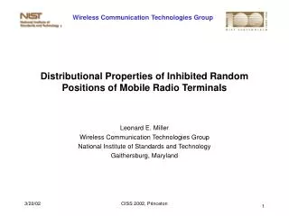
Distributional Properties of Inhibited Random Positions of Mobile Radio Terminals Leonard E. Miller Wireless Communication Technologies Group National Institute of Standards and Technology Gaithersburg, Maryland CISS 2002, Princeton
Abstract/Outline • Subject: Spatial distribution properties of randomly generated points representing the deployment of radio terminals (nodes) in an area. • Focus: Measures of area coverage, connectivity. • Focus: Influence of “inhibition” process that controls the minimum distance between nodes. • Cheng & Robertazzi, "A New Spatial Point Process for Multihop Radio Network Modeling," Proc. 1990 IEEE Internat'l Conf. on Comm., pp. 1241-1245. • Sampling of results relating measures of connectivity. CISS 2002, Princeton
Wireless Network Modeling What is the difference between these two random networks? CISS 2002, Princeton
Node positions are “inhibited” for one network • Both networks are generated using uniform distributions for x and y positions, but the second network adds the requirement or “inhibition” that nodes cannot be closer than R/D = x0 = 0.05. • The average number of neighbors per node is lower for the inhibition process in this example (4.41 vs. 3.34), but the average node-pair connectivity is higher (1.00 vs. 0.44) because the nodes are placed more evenly in the space. • Intuitively, the network with the minimum distance requirement also provides better “area coverage.” • In this paper, a measure of area coverage is developed that shows the effect of inhibition quantitatively. Also, expressions are given for the mean and variance of the average number of neighbors per node. CISS 2002, Princeton
Measures of Area Coverage • A measure of the area coverage of a random placement of N nodes in a D´D area can be based on the statistical variation of the number of nodes across regular subdivisions of the area, say "cells" of size D2/N. • On the average, for a random distribution of node locations, one would expect one node per cell. • The variance of the number of nodes per cell then would reflect the uniformity of the distribution of the node locations among the cells and hence the degree to which the node location process produces an even pattern of coverage for the area. CISS 2002, Princeton
Calculation of Area Coverage Measure Treat each cell as a trial, calculate mean and variance No inhibition dmin/D = 0.075 CISS 2002, Princeton
Binomial # nodes, n # cells Pn # cells Pn # cells Pn Pn 0 41 0.41 28 0.28 12 0.12 0.366 1 30 0.30 47 0.47 75 0.75 0.370 2 18 0.18 22 0.22 13 0.13 0.185 3 10 0.10 3 0.03 0 0.00 0.060 4 1 0.01 0 0.00 0 0.00 0.015 Sample mean 1.00 1.00 1.01 1.00 Sample variance 1.09 0.62 0.25 0.99 Results of calculation to test concept CISS 2002, Princeton
Probability of n nodes in a cell outside inside A: radius = minimum distance between nodes CISS 2002, Princeton
Analytical Expression for Pn where A = area around a selected node that is “inhibited.” For A = 0, CISS 2002, Princeton
Estimates using (2) Result, 1000 trials x0 A nmax Mean Variance Mean Variance 0.00 0.00 N 1.000 0.990 1.000 0.989 0.01 0.00029 100 1.000 0.962 1.000 0.960 0.02 0.00105 9 0.998 0.883 1.000 0.893 0.03 0.00215 5 0.999 0.777 1.000 0.793 0.04 0.00345 3 1.000 0.653 1.000 0.682 0.05 0.00483 3 1.002 0.520 1.000 0.576 0.06 0.00620 2 1.062 0.461 1.000 0.475 0.07 0.00745 2 1.134 0.407 1.000 0.387 0.075 0.00800 2 1.169 0.376 1.000 0.347 Comparison of Analysis, SimulationUsing A’ = E{A} CISS 2002, Princeton
Mean, Variance of # Neighbors • The simplest measure of connectivity is the average number of neighbors per node, n. • n = # connections (links) / # nodes • The analysis in this paper gives the mean value of n with and without inhibition in the selection of node locations. • The analytical values are compared to simulated values, plus empirical values of the variance of the number of neighbors are obtained. CISS 2002, Princeton
Conditional Mean and Variance • Conditioned on the location p of a particular node, the number of neighbors for the node is the result of N-1 binomial trials: E{n | p; x0} = (N-1) a(p; x0) Var{n | p; x0} = (N-1) a(p; x0) [1-a(p; x0)] where a(p) min{1, p(x2 – x02)} p Inhibited area Communications area CISS 2002, Princeton
Unconditional Mean and Variance where CISS 2002, Princeton
Example Simulation Results Results diverge from theory forx0 > 0because of sample size. CISS 2002, Princeton
Scaling of Mean: For 400 nodes (four times the node density), halve the range and the inhibition distance to get the same results for n CISS 2002, Princeton
Scaling of variance: inversely proportional to node density CISS 2002, Princeton
Further Work • Statistical relationship between #neighbors and connectivity, with and without inhibition • Means, variances • Correlation coefficients • Methods for generating “random” networks with specified connectivity CISS 2002, Princeton
Connectivity vs. #Neighbors--Relationship is statistical CISS 2002, Princeton
Connectivity vs. #Neighbors--Correlation is positive for low connectivity CISS 2002, Princeton
Connectivity vs. #Neighbors--Relation between averages CISS 2002, Princeton