Download
1 / 64
640 likes | 662 Vues
This document outlines the process of regularization for energy-based representations using stabilizing functions such as membrane stabilizers and thin plate stabilizers. The energy function measures compatibility between observations and data. The overall energy is minimized by finding the solution for u, obtained by minimizing E(u).

E N D
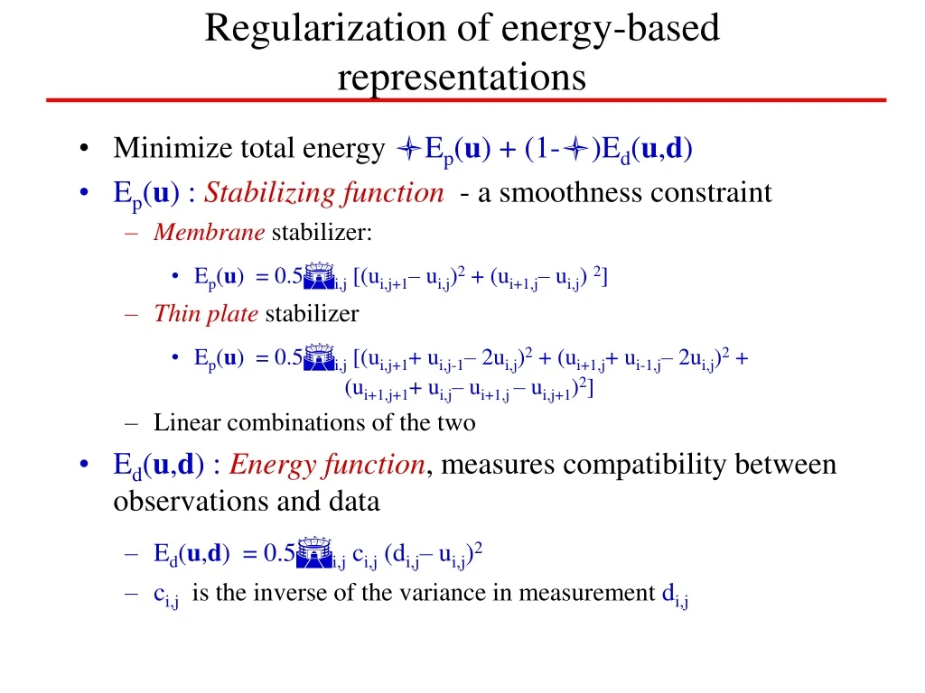
Regularization of energy-based representations • Minimize total energy lEp(u) + (1-l)Ed(u,d) • Ep(u) : Stabilizing function - a smoothness constraint • Membrane stabilizer: • Ep(u) = 0.5Si,j [(ui,j+1– ui,j)2 + (ui+1,j– ui,j) 2] • Thin plate stabilizer • Ep(u) = 0.5Si,j [(ui,j+1+ ui,j-1– 2ui,j)2 + (ui+1,j+ ui-1,j– 2ui,j)2 + (ui+1,j+1+ ui,j– ui+1,j – ui,j+1)2] • Linear combinations of the two • Ed(u,d) : Energy function, measures compatibility between observations and data • Ed(u,d) = 0.5Si,j ci,j (di,j– ui,j)2 • ci,j is the inverse of the variance in measurement di,j
Stabilizing function – membrane stabilizer Ep(u) = 0.5Si,j[ (ui,j+1– ui,j)2 + (ui+1,j– ui,j)2 ] ui,j i j
Stabilizing function – membrane stabilizer Ep(u) = 0.5Si,j[ (ui,j+1– ui,j)2 + (ui+1,j– ui,j)2 ] ui,j i j
Stabilizing function – membrane stabilizer Ep(u) = 0.5Si,j[ (ui,j+1– ui,j)2 + (ui+1,j– ui,j)2 ] ui,j i j
Stabilizing function – membrane stabilizer ATOM Ep(u) = 0.5Si,j[ (ui,j+1– ui,j)2 + (ui+1,j– ui,j)2 ] ui,j i j
Stabilizing function – membrane stabilizer ATOM • ui,jui,j + ui,j+1ui,j+1 – ui,jui,j+1 – ui,j+1ui,j Ep(u) = 0.5Si,j[ (ui,j+1– ui,j)2 + (ui+1,j– ui,j)2 ] ui,j i j 1 -1
Stabilizing function – membrane stabilizer ATOM • ui,jui,j + ui+1,jui+1,j – ui,jui+1,j – ui+1,jui,j Ep(u) = 0.5Si,j[ (ui,j+1– ui,j)2 + (ui+1,j– ui,j)2 ] ui,j i j -1 2 -1
Stabilizing function – membrane stabilizer ATOM • ui,jui,j + ui,j+1ui,j+1 – ui,jui,j+1 – ui,j+1ui,j Ep(u) = 0.5Si,j[ (ui,j+1– ui,j)2 + (ui+1,j– ui,j)2 ] ui,j i j -1 -1 3 -1
Stabilizing function – membrane stabilizer ATOM • ui,jui,j + ui+1,jui+1,j – ui,jui+1,j – ui+1,jui,j Ep(u) = 0.5Si,j[ (ui,j+1– ui,j)2 + (ui+1,j– ui,j)2 ] ui,j i j -1 -1 4 -1 -1
Stabilizing function – membrane stabilizer ATOM • ui,jui,j + ui+1,jui+1,j – ui,jui+1,j – ui+1,jui,j Ep(u) = 0.5Si,j[ (ui,j+1– ui,j)2 + (ui+1,j– ui,j)2 ] ui,j i j -1 -1 4 -1 -1 = u
Stabilizing function – membrane stabilizer ATOM • ui,jui,j + ui+1,jui+1,j – ui,jui+1,j – ui+1,jui,j Ep(u) = 0.5Si,j[ (ui,j+1– ui,j)2 + (ui+1,j– ui,j)2 ] ui,j i j -1 -1 4 -1 -1 = u • Ep(u) = 0.5uTApu • Rows of Ap have the form • 0 0 0 –1 0 0 …. 0 –1 4 –1 0 … 0 0 –1 0 ..
Stabilizing function – thin plate stabilizer Ep(u) = 0.5Si,j{[(ui,j+1– ui,j) + (ui,j-1– ui,j)]2 + [(ui+1,j– ui,j) + (ui-1,j– ui,j)]2+ 2[(ui+1,j+1– ui,j) + (ui,j– ui+1,j) + (ui,j–ui,j+1)]2} ui,j i j
Stabilizing function – thin plate stabilizer Ep(u) = 0.5Si,j{[(ui,j+1– ui,j) + (ui,j-1– ui,j)]2 + [(ui+1,j– ui,j) + (ui-1,j– ui,j)]2+ 2[(ui+1,j+1– ui,j) + (ui,j– ui+1,j) + (ui,j–ui,j+1)]2} ui,j i j
Stabilizing function – thin plate stabilizer Ep(u) = 0.5Si,j{[(ui,j+1– ui,j) + (ui,j-1– ui,j)]2 + [(ui+1,j– ui,j) + (ui-1,j– ui,j)]2+ 2[(ui+1,j+1– ui,j) + (ui,j– ui+1,j) + (ui,j–ui,j+1)]2} ui,j i j
Stabilizing function – thin plate stabilizer Ep(u) = 0.5Si,j{[(ui,j+1– ui,j) + (ui,j-1– ui,j)]2 + [(ui+1,j– ui,j) + (ui-1,j– ui,j)]2+ 2[(ui+1,j+1– ui,j) + (ui,j– ui+1,j) + (ui,j–ui,j+1)]2} ui,j i j
Stabilizing function – thin plate stabilizer Ep(u) = 0.5Si,j{[(ui,j+1– ui,j) + (ui,j-1– ui,j)]2 + [(ui+1,j– ui,j) + (ui-1,j– ui,j)]2+ 2[(ui+1,j+1– ui,j) + (ui,j– ui+1,j) + (ui,j–ui,j+1)]2} ui,j i j 1 -8 2 2 ATOM: 1 -8 -8 1 20 -8 2 2 1 • Ep(u) = 0.5uTApu • Rows of Ap have the form • 0 0 1 0 0 ... 0 2 –8 2 0 0 .. 1 –8 20 –8 1 0 0 …0 0 2 –8 2 0 .. 0 –1 0 ..
Stabilizing function – Examples (1-D) points membrane thin plate thin plate + membrane
Stabilizing function – Examples (2-D) membrane Samples from u thin plate membrane + thin plate
Stabilizing function – Examples (2-D) membrane Samples from u thin plate membrane + thin plate
Energy function • Data on grid • di,j= ui,j +ei,j (ei,j is N(0,s2)) • Ed(u,d) = 0.5Si,j ci,j (di,j– ui,j)2 (ci,j = s-2) • Data off grid • dk = h0,0 ui,j +h0,1 ui,j+1 + h1,0 ui+1,j + h1,1 ui+1,j+1 +ei,j • Ed(u,d) = 0.5Sk ck (dk,– Hku)2 • In all examples here we assume data on grid • Ed(u,d) = 0.5 (u-d)TAd(u-d) • Ad = s-2 I : measurement variance assumed constant for all data
Overall energy • E(u) = lEp(u) + (1-l)Ed(u,d) (l isregularization factor) = 0.5{luTApu + (1-l)(u-d)TAd(u-d)} = 0.5uTAu – uTb + const • Where A = Ap + (1-l)Ad b = (1-l) Ad d • Solution for u can be directly obtained by minimizing E(u) u = A-1 b
Minimizing overall energy 1-D (l = 0.5) From noisy observation membrane No observation noise From noisy observation thin plate No observation noise
Minimizing overall energy 2-D (l = 0.5) Original Noisy Added 0 mean unit variance Gaussian noise to all elements
Minimizing overall energy 2-D (l = 0.5) Original From Noisy membrane thin plate
Minimizing overall energy 2-D (l = 0.5) Original Noisy Added 0 mean unit variance Gaussian noise to all elements
Minimizing overall energy 2-D (l = 0.5) Original From Noisy membrane thin plate
Minimizing energy by Relaxation • Direct computation of A-1is inefficient • Large matrices: for a 256x256 grid, Ahas size 65536 x 65536 • Sparseness of A not utilized: only a small fraction of elements have non zero values • Relaxation replaces inversion of A with many local estimates ui+ = ai,i-1(bi – Sai,juj) • Updates can be done in parallel • All local computations very simple • Can be slow to converge
Minimizing energy by relaxation 1-D (l = 0.5) Membrane 100 iters 500 iters 1000 iters
Minimizing energy by relaxation 1-D (l = 0.5) Thin plate: much slower to converge 1000 iters 10000 iters 100000 iters
Minimizing energy by relaxation 2-D (l = 0.5) Original 1000 iters Membrane 10000 iters 100000 iters
Minimizing energy by relaxation 2-D (l = 0.5) Original 1000 iters Thin plate: much slower to converge 10000 iters 100000 iters
Prior Models • A Boltzmann distribution based on the stabilizing function P(u) = K.exp(-Ep(u)/Tp) • K is a normalizing constant, Tp is temperature • Samples can be generated by repeated sampling of local distributions: P(ui|u) • P(ui|u) = Ziexp(-ai,i-1(ui – ui+)/2Tp) • ui+ = ai,i-1(bi – Sai,juj) • This is the local estimate of ui in the relaxation method • The variance of the local sample is Tp/ai,i
Samples from prior distribution 1-D Membrane stabilizer based Boltzmann Thin plate stabilizer based Boltzmann
Samples from prior distribution 2-D Membrane prior
Samples from prior distribution 2-D Thin plate prior
Sampling prior distributions • Samples are fractal • Tend to favour high frequencies • Multi-grid sampling to get smoother samples: Initially generate sample for a very coarse grid
Sampling prior distributions • Samples are fractal • Tend to favour high frequencies • Multi-grid sampling to get smoother samples: Interpolate from coarse grid to finer grid, use the interpolated values to initilize gibbs sampling for a less coarse grid.
Sampling prior distributions • Samples are fractal • Tend to favour high frequencies • Multi-grid sampling to get smoother samples: Repeat process on a finer grid
Sampling prior distributions • Samples are fractal • Tend to favour high frequencies • Multi-grid sampling to get smoother samples: Final sample for entire grid
Multigrid sampling of prior distribution Membrane prior Thin plate prior
Sensor models • Sparse data model • Uses a simple energy function • Assumption: data points are all on grid • Only use sparse data model used in examples • Others such as force field models, optical flow, image intensity etc. not simulated for this presentation • Measurement variance assumed constant for all data points
Posterior model • Simple Bayes’ rule: P(u|d) = K.exp(-Ep(u)/Tp - Ed(u)) • Also a Gibbs distribution • 1/Tp is the equivalent of the regularization factor Tp = (1-l)/ l • In following figures only thin plate prior considered
MAP estimation from the Gibbs posterior • Restate Gibbs posterior distribution as P(u) = K.exp(-E(u)/T) • E(u) is the total energy • T again is temperature • Not to be confused with regularization term Tp • Reduce T with iterations • iteration is defined as a complete sweep through the data • Guaranteed convergence to MAP estimate as T goes to 0, provided T does not go down faster than 1/log(iter), where iter is the iteration number • In practice, much faster cooling is possible • For simple sparse data sensor model, MAP estimate must be identical to that obtained using relaxation or matrix inversion
MAP estimates from posterior 1-D Relaxation 100000 iters Annealed Gibbs sampling 100000 iters
MAP estimates from posterior 2-D Actual MAP solution Annealed Gibbs Sampling based MAP solution
The contaminated Gaussian sensor model • Also a sparse data sensor model • Assumes measurement error has two modes • 1. A high probability, low variance Gaussian • 2. A low probability, high variance Gaussian P(di,j |u) = (1-e)N(ui,j ,s12) + e N(ui,j , s22) • 0.05 < e < 0.1 and s22 >> s12 • Posterior probability is also a mixture of Gaussians (1-e)P1(di,j |u) + eP2(di,j |u)
MAP estimates of contaminated Gaussian 1-D • For contaminated Gaussian there is no closed form estimate MAP estimate • Gibbs sampling provides a MAP estimate MAP estimate using single Gaussian sensor model MAP estimate using contaminated Gaussian sensor model
MAP estimates of contaminated Gaussian 2-D MAP estimate using a single Gaussian sensor model MAP estimate using a contaminated Gaussian sensor model • For contaminated Gaussian MAP estimate obtained using annealed Gibbs sampling