Download

1 / 20
200 likes | 425 Vues
Bifurcations and attractors of a model of supply and demand. Siniša Slijepčević 22 February 2008 PMF – Deparment of Mathematics. CONTENTS. Introduction to dynamical systems Example of a model of supply and demand – residential real estate market in Croatia Conclusions. MOTIVATION.

E N D
Bifurcations and attractors of a model of supply and demand Siniša Slijepčević 22 February 2008 PMF – Deparment of Mathematics
CONTENTS • Introduction to dynamical systems • Example of a model of supply and demand – residential real estate market in Croatia • Conclusions
MOTIVATION • Theory of dynamical systems in economical modeling: • Theory of dynamical systems is used to model and explain deterministic phenomena, without elements of randomness • The theory can model complex looking phenomena with relatively simple models • Key tricks • Lots of tricks to deduce and explain behavior of a model without solving it explicitly • Developed theory to understand changes of behavior of a class of models, depending on a parameter (attractors, bifurcations) Typical phase portrait of a 2D model
ORBITS OF THE PREDATOR-PREY MODEL (1/2) “Periodic” behavior for the value of the parameter p = 1.5 f(x) x
ORBITS OF THE PREDATOR-PREY MODEL (2/2) “Chaotic” behavior for the value of the parameter p = 3.9 f(x) x
BIFURCATION DIAGRAM OF THE PREDATOR – PREY MODEL Attractor of the dynamical system for each parameter, period doubling bifurcation Phase space X=[0,1] Parameter r
CONTENTS • Introduction to dynamical systems • Example of a model of supply and demand – residential real estate market in Croatia • Conclusions
FACTS REGARDING THE RESIDENTIAL REAL ESTATE MARKET IN CROATIA • Number of flats being put on the market in Zagreb • Currently more than 60,000 people look for an appartment • Current oversupply of over 2000 flats • Is the market working ? 6139 4771 4015 4627 3341 2006 2005 2004 2003 2002 Source: CBRE
DECISION MAKING MODEL OF A TYPICAL DEVELOPER • Sanitized investment plan of a leading European developer for a residential project in Zagreb
KEY PARAMETERS IN THE DECISION MAKING PROCESS OF A TYPICAL DEVELOPER TO BUILD A RESIDENTIAL BLOCK IN ZAGREB • Sales price / sqm (analysis in practice based on the current sales price) • Cost of land / sqm • Cost of construction / sqm • Communal and water tax / sqm • Cost to finance (i.e. interest rates; likely leverage) Developers discriminated by the cost of construction and cost to finance
DECISION MAKING MODEL OF A TYPICAL RESIDENTIAL BUYER Example Factor 12,000 kn Income of the family: Disposable income: 25 % of the income 60 sqm Required sqm: Loan (number of years): 30 years Max price / sqm: 2,300 Euro / sqm
SUPPLY – DEMAND CURVE FOR RESIDENTIAL REAL ESTATE • Conceptual Price / sqm Euro Supply (by developer group) Demand 3000 2500 2000 1500 10000 5000 0 Number of flats developed / year
KEY IDEAS FOR MODELING DYNAMICAL SUPPLY AND DEMAND xn – the price of the residential real estate / sqm (Euro), 1 Jan of each year Variables: ln – the price of the residential zoned land / sqm (Euro), 1 Jan of each year xn+1 = r xn (1 – xn) bn – number of flats put on market in each year (pre sales) i.e. the “normalized” price of the residential real estate behaves accordingly to a predator – prey model r – proportional to interest rates and average construction cost / sqm Parameter: Key principles: • Model everything in “nominal”, normalized terms, i.e. net of nominal GDP growth • Assume growth of income distribution proportional to GDP growth; i.e. constant in the model
BIFURCATION DIAGRAM FOR THE MODEL OF THE RESIDENTIAL REAL ESTATE SUPPLY AND DEMAND IN TIME Normalized price of the residential real estate / year Parameter r 2004: r ~ 2.71 Attractor: stable growth 2004: r ~ 3.62 Attractor: Period 4
CONTENTS • Introduction to dynamical systems • Example of a model of supply and demand – residential real estate market in Croatia • Conclusions
EXAMPLE – COMPLEX MODELING OF SUPPLY AND DEMAND • Model of energy supply and demand in two regions in China • X(t) – Energy supply in the region A • Y(t) – Energy demand in the region B • Z(t) – Energy import from the region A to the region B • Lorenz – type chaotic attractor • Phenomenologically equivalent behavior to a much simpler predator – prey model Source: Mei Sun, Lixin Tian, Ying Fu; Chaos, Solitons, Fractals 32 (2007)
QUESTIONS FOR FURTHER ANALYSIS • Does the model faithfully represent behavior of the real estate market in a longer period of time in Croatia? (to be checked experimentally) • Can it be implemented to other markets (e.g. the US)? • Which policy is optimal to “regulate” the market, i.e. prevent the real estate prices bifurcating into the chaotic region? • Regulating supply (i.e. the POS – type policy?) • Regulating demand (i.e. the loan interest subsidies for the first time purchasers)? • Regulating land prices; e.g. by putting Government owned or Municipal land for sale or “right to build” for residential development, for preferential prices?