From a problem to program
This piece explores the transition from scientific problems to computational solutions, emphasizing the importance of mathematical models, numerical algorithms, and computer programming. Key topics include the distinction between well-posed and ill-posed problems, sources of numerical errors such as rounding and truncation, and methods to mitigate these issues. Additionally, it highlights the significance of error estimation, data accuracy, and the implications of floating-point representation in computations. The content aims to guide readers in the reliable solution of numerical problems via proper modeling and error management techniques.


From a problem to program
E N D
Presentation Transcript
From a problem to program • Scientific problem • Mathematical model: exact, often continuous functions • Numerical, computational model • algorithms • Computer programs • Profiling of the program • Computation • Error estimation • Analysis of results
Sources of error • Mathematical model: too simple, not flexible enough • Numerical errors: discretization, truncation • Errors in data: statistical, systematic • Problems in the algorithms: numerical instability • Rounding errors
Well- and ill-posed problems • A task is well-posed, if the solution • Exist for all starting values • Is unique • Is stable for all initial values • Ill posed problem does not have these properties.
Well- and ill-posed problems • Solutions of well-posed problems are good approximations of the exact solution. • An ill-posed problem cannot be solved reliably and exactly. • There are special methods for ill-posed problem which give agreeable solutions.
Integers • Integers are exact in a computer. • Integers are presented with a fixed number of bits. • The largest and smallest integer exists. Overflow can happen. • The number of bits is usually a certain numbers of bytes (8 bits). • Examples: 2 bytes(16 bits), 4 bytes (32 bits), or even 8 bytes (64 bits). • In many systems the number of bytes can be chosen.
Integers (kokonaisluvut) • different presentations, the order of bits varies • Example two’s complement n bits, smallest -2n-1 and largest2 n-1-1
Floating point numbers (liukuluvut) • Floating point numbers are approximations to real numbers. • A floating point number consist of two integers, mantissa m and exponent e, which both include a sign (positive or negative). As a formula f=m2e. • Thus the smallest (fmin) and largest (fmax) floating point number exists. Floating point numbers are not distributed evenly at interval (fmin, fmax). • In principle the base does not need to be 2.
From real number to a floating point number • Truncation or rounding • Numbers are truncated also in arithmetic operations. • Programming languages usually allow one to choose the precision, for instance 32 or 64 bits. • IEEE: mantissa24 bits andexponent 8 bits. • Largest floating point number1038 and smallest positive floating point number is10-38.
Overflow or underflow • Overflow occurs when one exceeds the largest floating point number. Underflow occurs with anything smaller than the smallest floating point number. • Overflow can sometimes be avoided by reformulating the equation. • Examplean/bn = (a/b)n • Sometimes scaling the variables can help. • If -statements
Matlab REALMAX Largest positive floating point number. x = realmax is the largest floating point number representable on this computer. Anything larger overflows. REALMIN Smallest positive floating point number. x = realmin is the smallest positive normalized floating point number on this computer. Anything smaller underflows or is an IEEE "denormal".
Matlab (a/b)^n or a^n/b^n? >> a=5; b=3; n = log(realmax)/log(a/b) % choose a,b n = % compute n 1.3895e+03 >> (a/b)^n % gives result ans = 1.7977e+308 >> a^n/b^n % does not work ans = NaN
Rounding errors • A floating point number is only an approximation for a real number: rounding errors cannot be avoided. • Rounding errors occurs in the input of data and in computations. • Minimize the amount of arithmetic operations. • Round only the final results. • Use large precision.
Rounding errors • summations and iterations • It is dangerous to compare directly the values of two floating point variables. It is better to test that their difference is smaller than a given limit. Example.Comparison of two floating point numbersa and b. Not good if a = b.Better: if abs(a-b) < epsilon, where epsilon is a suitable value.
Cancellation error • Occurs when two floating point numbers are large compared to their precision. • When the difference of the two numbers is about the same as the precision of the more inaccurate number, it is not accurate enough. • This kind of error is called thecatastrophic cancellation (kumoutumisvirhe).
Example • Two floating point numbers x and y, and their errosDx and Dy. • If x=0.5554 and y=0.5553, and the errors Dx = Dy = 0.00005, then the difference is x-y=0.0001. The error for the difference would be 0.00007! (Dahlquist and Björk 1974)
Matlab: » x = 0.5554; y= 0.5553; » x-y » ans = 1.0000e-004 »dx = 0.00005; dy = dx; » % law of propagation of errors » sqrt(dx^2+dy^2) ans = 7.0711e-005
Esimerkki • Laskettaessa yhteen hyvin suuri ja pieni luku voi käydä niin, että pienempiluku on samaa suuruusluokkaa kuin suuremman luvun tarkkuus, jolloinpienemmällä luvulla ei ole mitään vaikutusta lopputulokseen. • Ratkaisunatähänkin ongelmaan on useinalgoritmin vaihto eli laskukaavan saattaminen johonkinmuuhun matemaattisesti ekvivalenttiin, mutta numeerisesti erilaiseen muotoon.
Example • Sum of alternating serie exp(-x) = 1/exp(x) • Numerical derivative (f(x+h)-f(x))/h
Scaling • Peruslaskutoimituksia pitäisi suorittaa mieluiten luvuilla, jotkaovat keskenään samaa suuruusluokkaa ja järkevän suuruisiaverrattuina lukualueeseen ja liukulukujen tarkkuuteen. • Ongelmajoudutaan usein skaalaamaan, jotta pysyttäisiin liukulukualueenrajoissa.
Skaalaus • Muuttujat eivät saisi olla laadullisia suureita. • Laaduttomiin suureisiinpäästään jakamalla tällaiset muuttujat sopivilla probleemaan liittyvillä'mittatikuilla', jotka muuntavat muuttujien arvot järkevän suuruisiksi. • Käyttäjäystävällinen ohjelma tekee tietenkin skaalaukset sisäisesti.Syöttödata annetaan sille fysikaalisissa yksiköissä ja se palauttaa myöstulokset näissä yksiköissä. Muunnokset tapahtuvat siis juuri ennentulostusta ja syötön jälkeen.
Discretization • Discretization means estimation of a continuous function with discrete function with a limited number of points. • This causes the so called discretization error.
Truncation • For simplicity consider a function of one variable f(x). • In computer the function must be truncated to a finite interval a<x<b. • The results may inaccurate if the function f is not zero outside the interval (a,b).
Integration of Lorenz function >> f = inline(’1./(1+x.^2)’, ’x’); >> quad(f,-10,10) ans = 2.9423 >> quad(f,-100,100) ans = 3.1216 >> quad(f,-1000,1000) ans = 3.1396 >> quad(f,-100000,100000) ans = 3.1416 vrt. vanha versio antaa 65.1343!!!
Discretization • Interval (a,b) is divided to subintervals {a=x1< x2<…< xN = b}. • The discrete approximation of the function is a set of its values {f(a) =f(x1), f(x2),…, f(xN) = f(b)}. • Choosing the points x1,x2,…,xNis crucial for the accuracy of the results.
Trapezoidal formula for integration • Integrate f(x) from at interval (a,b) • Choose the points {a=x1, x2,…,xN=b}. • Replace the integral by the sum Σi½ (f(xi)-f(xi-1)) (xi-xi-1)
Lorenz function, integration trapezoidal formula (puolisuunnikassääntö) x =-10:0.1:10; trapz(x,f(x)) ans = 2.9423 x =-1000:0.1:1000; trapz(x,f(x)) ans = 3.1396 x = -1000:1:1000; trapz(x,f(x)) ans = 3.1513
Numerical derivative • Mathematically the derivative of the function f is the limit (f(x+h)-f(x))/h when h approaches to zero. • Numerical approximation of the derivative f’(xi) ≈ (f(xi+1) –f(xi))/(xi+1–xi)
Numerical derivative » x = 0:0.1:4*pi; h=0.1; subplot(1,2,1), plot(x+h/2,(cos(x+h)-cos(x))/h,x,-sin(x),'.') » x = 0:0.5:4*pi; h=0.5; subplot(1,2,2), plot(x+h/2,(cos(x+h)-cos(x))/h,x,-sin(x),'.')
Important • Matemaattisesti ekvivalentitalgoritmit (antaisivat samat tulokset, jos laskentatarkkuus olisi ääretön jalaskentaan käytettävät resurssit olisivat äärettömät) eivät juuri koskaan anna samojatuloksia eivätkä ole juuri koskaan yhtä tehokkaita. • Mathematically equivalent algorithms do not usually give the same results and are not equally effective.