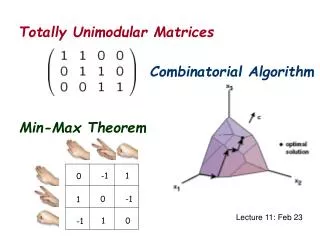
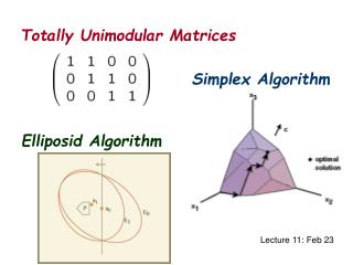
Totally Unimodular Matrices

1. Totally Unimodular Matrices Simplex Algorithm Elliposid Algorithm Lecture 11: Feb 23

2. Integer Linear programs Method: model a combinatorial problem as a linear program. Goal: To prove that the linear program has an integer optimum solution for every objective function. Goal: Every vertex (basic) solution is an integer vector. • Consequences: • The combinatorial problem (even the weighted case) is polynomial time solvable. • Min-max theorems for the combinatorial problem through the LP-duality theorem.

3. Method 1: Convex Combination A point y in Rn is a convex combination of if y is in the convex hull of Fact: A vertex solution is not a convex combination of some other points. Method 1: A non-integer solution must be a convex combination of some other points. Examples: bipartite matching polytope, stable matching polytope.

4. Method 2: Linear Independence Tight inequalities: inequalities achieved as equalities Vertex solution: unique solution of n linearly independent tight inequalities Think of 3D. Method 2: A set of n linearly independent tight inequalities must have some tight inequalities of the form x(e)=0 or x(e)=1. Proceed by induction. Examples: bipartite matching polytope, general matching polytope.

5. Method 3: Totally Unimodular Matrices m constraints, n variables Vertex solution: unique solution of n linearly independent tight inequalities Can be rewritten as: That is:

6. Method 3: Totally Unimodular Matrices Assuming all entries of A and b are integral When does has an integral solution x? By Cramer’s rule where Ai is the matrix with each column is equal to the corresponding column in A except the i-th column is equal to b. x would be integral if det(A) is equal to +1 or -1.

7. Method 3: Totally Unimodular Matrices A matrix is totally unimodular if the determinant of each square submatrix of is 0, -1, or +1. Theorem 1: If A is totally unimodular, then every vertex solution of is integral. Proof (follows from previous slides): • a vertex solution is defined by a set of n linearly independent tight inequalities. • Let A’ denote the (square) submatrix of A which corresponds to those inequalities. • Then A’x = b’, where b’ consists of the corresponding entries in b. • Since A is totally unimodular, det(A) = 1 or -1. • By Cramer’s rule, x is integral.

8. Example of Totally Unimodular Matrices A totally unimodular matrix must have every entry equals to +1,0,-1. Guassian elimination And so we see that x must be an integral solution.

9. Example of Totally Unimodular Matrices is not a totally unimodular matrix, as its determinant is equal to 2. x is not necessarily an integral solution.

10. Method 3: Totally Unimodular Matrices Primal Dual Transpose of A Theorem 2: If A is totally unimodular, then both the primal and dual programs are integer programs. Proof: if A is totally unimodular, then so is it’s transpose.

11. Application 1: Bipartite Graphs Let A be the incidence matrix of a bipartite graph. Each row i represents a vertex v(i), and each column j represents an edge e(j). A(ij) = 1 if and only if edge e(j) is incident to v(i). edges vertices

12. Application 1: Bipartite Graphs We’ll prove that the incidence matrix A of a bipartite graph is totally unimodular. Consider an arbitrary square submatrix A’ of A. Our goal is to show that A’ has determinant -1,0, or +1. Case 1: A’ has a column with only 0. Then det(A’)=0. Case 2: A’ has a column with only one 1. By induction, A’’ has determinant -1,0, or +1. And so does A’.

13. Application 1: Bipartite Graphs Case 3: Each column of A’ has exactly two 1. +1 We can write -1 Since the graph is bipartite, each column has one 1 in Aup and one 1 in Adown So, by multiplying +1 on the rows in Aup and -1 on the columns in Adown, we get that the rows are linearly dependent, and thus det(A’)=0, and we’re done. +1 -1

14. Application 1: Bipartite Graphs Maximum bipartite matching Incidence matrix of a bipartite graph, hence totally unimodular, and so yet another proof that this LP is integral.

15. Application 1: Bipartite Graphs Maximum general matching The linear program for general matching does not come from a totally unimodular matrix, and this is why Edmonds’ result is regarded as a major breakthrough.

16. Application 1: Bipartite Graphs Theorem 2: If A is totally unimodular, then both the primal and dual programs are integer programs. Maximum matching <= maximum fractional matching <= minimum fractional vertex cover <= minimum vertex cover Theorem 2 show that the first and the last inequalities are equalites. The LP-duality theorem shows that the second inequality is an equality. And so we have maximum matching = minimum vertex cover.

17. Application 2: Directed Graphs • Let A be the incidence matrix of a directed graph. • Each row i represents a vertex v(i), • and each column j represents an edge e(j). • A(ij) = +1 if vertex v(i) is the tail of edge e(j). • A(ij) = -1 if vertex v(i) is the head of edge e(j). • A(ij) = 0 otherwise. The incidence matrix A of a directed graph is totally unimodular. • Consequences: • The max-flow problem (even min-cost flow) is polynomial time solvable. • Max-flow-min-cut theorem follows from the LP-duality theorem.

18. Black Box Problem Solution Polynomial time LP-formulation Vertex solution LP-solver integral

19. Simplex Method Simplex method: A simple and effective approach to solve linear programs in practice. It has a nice geometric interpretation. Idea: Focus only on vertex solutions, since no matter what is the objective function, there is always a vertex which attains optimality.

20. Simplex Method • Simplex Algorithm: • Start from an arbitrary vertex. • Move to one of its neighbours • which improves the cost. Iterate. Key: local minimum = global minimum Global minimum Moving along this direction improves the cost. There is always one neighbour which improves the cost. We are here

21. Simplex Method • Simplex Algorithm: • Start from an arbitrary vertex. • Move to one of its neighbours which improves the cost. Iterate. Which one? There are many different rules to choose a neighbour, but so far every rule has a counterexample so that it takes exponential time to reach an optimum vertex. MAJOR OPEN PROBLEM: Is there a polynomial time simplex algorithm?

22. Simplex Method For combinatorial problems, we know that vertex solutions correspond to combinatorial objects like matchings, stable matchings, flows, etc. So, the simplex algorithm actually defines a combinatorial algorithm for these problems. For example, if you consider the bipartite matching polytope and run the simplex algorithm, you get the augmenting path algorithm. The key is to show that two adjacent vertices are differed by an augmenting path. Recall that a vertex solution is the unique solution of n linearly independent inequalities. So, moving along an edge in the polytope means to replace one tight inequality by another one. There is one degree of freedom and this corresponds to moving along an edge.

23. Ellipsoid Method Goal: Given a bounded convex set P, find a point x in P. Key: show that the volume decreases fast enough • Ellipsoid Algorithm: • Start with a big ellipsoid which contains P. • Test if the center c is inside P. • If not, there is a linear inequality ax <=b for which c is violated. • Find a minimum ellipsoid which contains the intersection of the previous ellipsoid and ax <= b. • Continue the process with the new (smaller) ellipsoid.

24. Ellipsoid Method Goal: Given a bounded convex set P, find a point x in P. Why it is enough to test if P contains a point??? Because optimization problem can be reduced to this testing problem. Any point which satisfies this new system is an optimal solution of the original system.

25. Ellipsoid Method Important property: We just need to know the previous ellipsoid and a violated inequality. This can help to solve some exponential size LP if we have a separation oracle. Separation orcale: given a point x, decide in polynomial time whether x is in P or output a violating inequality.

26. Application of the Ellipsoid Method Maximum matching To solve this linear program, we need a separation oracle. Given a fractional solution x, the separation oracle needs to determine if x is a feasible solution, or else output a violated inequality. For this problem, it turns out that we can design a polynomial time separation oracle by using the minimum cut algorithm! For each odd set S, exponentially many!

27. What We Have Learnt (or Heard) Stable matchings Bipartite matchings Minimum spanning trees General matchings Maximum flows Shortest paths Minimum Cost Flows Submodular Flows Linear programming

28. What We Have Learnt (or Heard) How to model a combinatorial problem as a linear program. See the geometric interpretation of linear programming. How to prove a linear program gives integer optimal solutions? • Prove that every vertex solution is integral. • By convex combination method. • By linear independency of tight inequalities. • By totally unimodular matrices. • By iterative rounding (to be discussed). • By randomized rounding (to be discussed).

29. What We Have Learnt (or Heard) How to obtain min-max theorems of combinatorial problems? LP-duality theorem, e.g. max-flow-min-cut, max-matching-min-vertex-cover. See combinatorial algorithms from the simplex algorithm, and even give an explanation for the combinatorial algorithms (local minimum = global minimum). We’ve seen how results from combinatorial approach follow from results in linear programming. Later we’ll see many results where linear programming is the only approach we know of!