
Abstract
Conclusions By starting with magnitude distribution, we assure agreement with observed statewide distribution.

Abstract
E N D
Presentation Transcript
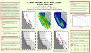
Conclusions • By starting with magnitude distribution, we assure agreement with observed statewide distribution. • 2. Length, width, and slip scaling assumes self similarity: constant ratio of length, width, and slip; all proportional to cube root of moment. Area scaling consistent with 2008 Working Group model. • 3. Weighting procedure puts largest earthquakes near major faults, with focal mechanisms consistent with fault orientation. • 4. Allows for rare surprises: large off-fault earthquakes, earthquakes over magnitude 8. • 5. Simple; no explicit stress calculation, no explicit fault-to-fault jumps. But rupture length may exceed fault length. Abstract We are constructing an earthquake source model for the UCERF3 project. The basic philosophy is to start with the things we know best: the magnitude distribution for the whole state, Omori’s law, total moment rate, distribution of moment rate on major faults, the instrumentally recorded earthquake catalog, long-term strain rate, historic earthquake catalog, and paleo-event catalog, in that order. The model is expressed as earthquake rate per unit area, time, magnitude, and focal mechanism direction, with algorithms to simulate “realized” earthquakes at random. The simulated earthquakes are described as spatially tapered ruptures on hypothetical rectangular fault planes with length, width, depth, strike, dip, and rake specified. Earthquake locations and orientations will approximate those of mapped faults based on empirical studies of actual earthquakes. The simulation scheme will allow temporal and spatial clustering according to the Critical Branching Model of Kagan et al. [2007] We would identify testable features of the models and devise quantitative prospective and/or retrospective tests as appropriate. We include a rule associating earthquakes with mapped faults based on the proximity of their hypocenters to those faults. In that way we can model fault slip rate and paleoseismic dates and displacements. California Earthquake Rupture Model Satisfying Accepted Scaling Laws(SCEC 2010, 1-129)David Jackson, Yan Kagan and Qi WangDepartment of Earth and Space Sciences, University of California Los Angeles • Procedure • Choose random magnitude from Tapered Gutenberg-Richter (Kagan) magnitude with corner magnitude 8.2. • 2. Assign average length, width, and slip from assumed scaling relationship. • 3. Choose random hypocenter location from normalized probability map • a. Weighted version two maps: one based on past earthquakes, • another on fault moment rates. • b. Weighting is linearly proportional magnitude: 100% earthquake • map at m=6.5; 100% fault map at m=8.5. • 4. Choose random focal mechanism from normalized probability map • a. Weighted version two maps: one based on past earthquakes, • another on fault moment rates. • b. Weighting is linearly proportional magnitude: 100% earthquake • map at m=6.5; 100% fault map at m=8.5. • 5. Resolve fault plane – auxiliary plane ambiguity based on nearby faults. Figure 7. Magnitude distribution of simulated earthquakes. Figure 2. Earthquake probability based on smoothed seismicity Figure 1. Extended sources representing large earthquakes in California Figure 3. Earthquake probability based on faults Simple scaling model for length, width, and slip VS. magnitude Kagan [2002] studied aftershock zone length vs moment for large shallow earthquakes in the CMT catalog. This study used the most accurate, comprehensive, and internally consistent data available. He concluded that length is proportional to the cube root of moment, which implies that width and slip scale the same way. Otherwise, one of them increases less strongly with moment and the other more strongly. For either that would pose the problem of "inverse saturation.“ Assuming the self=similarity implied by the Kagan result, we adopted the following forms for average length (L), average down-dip width (W) and average slip (D) as a function of moment magnitude (m): Log10(L) = a + 0.5*m L in km; a = -1.65 from Kagan [2002] Log10(D) = c + 0.5*m D in m; c = -3.50 from Wells and Coppersmith [1994] Log10(W) = b + 0.5*m W in km; b = -2.55 from m*L*W*D = 10^(1.5*m+9) We took m to be 5*1010 Nm. The sum a + b = -4.2 represents the area scaling, and it coincidentally equals the value used in the “Ellsworth B” magnitude-area relationship. The results: Data The earthquake catalog used for seismicity calculation covers 1800 to 2009 with minimum magnitude 4.7 and maximum depth 30 kilometers. This catalog was compiled by us from several previous catalogs. We selected the most reliable location and magnitude from the catalogs, and used regression relations to estimate the moment magnitude for each earthquake. Compared to previous catalogs, ours is more complete and includes more accurate magnitudes and hypocenter locations. The fault information is derived from the SCEC Community Fault Model, modified for the Uniform California Earthquake Rupture Forecast, and provided to us by Kevin Milner. For distance from fault calculations we simplified faults to line sources, at a depth of 7.5km in most cases. Figure 6. Simulated earthquakes and their ruptures. Rectangles represent ruptures of earthquake larger than 7.5. Single lines show the ruptures of other events. Figure 4. Smoothed focal mechanisms based on seismicity Figure 5. Smoothed focal mechanisms based on faults


