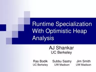
Runtime Specialization With Optimistic Heap Analysis

1. Runtime Specialization With Optimistic Heap Analysis AJ Shankar UC Berkeley

2. Specialization (partial evaluation) Code Constant Input • Hardcode constant values directly into the code • Big speedups (100%+) possible • But hard to make useable… Output Variable Input Specializer Code’ Output

3. First practical specializer Automatic: no manual annotations Dynamic: no offline phase Easy to deploy: hidden in a JIT compiler Powerful: precisely finds all heap constants Fast: under 1s, low overheads

4. Specializer: what would benefit? • Any program that relies heavily on data that is (largely) constant at runtime • For this talk, we’ll focus on one domain • But we’ve benchmarked several • Speedups of 20% to 500%

5. The local bookstore… JavaScript LISP Matlab Perl Python Ruby Visual Basic Scheme

6. Interpreters • Interpreters: preferred implementation • Easy to write • Verifiable: interpreter is close to the language spec • Deployable: easily portable • Programmer-friendly: enable rapid development cycle • More scripting languages to come • More interpreters to appear

7. But interpreters are slow • Programmers complain about interpreter speed • 20 open Mozilla bugs decrying slow JavaScript • Google searches: • “python slow”: 674k • “visual basic slow”: 3.1M • “perl slow”: 810k • (“perl porn”: 236k) • Compiler? • Time-consuming to write, maintain, debug • Programmers often don’t want one

8. Specialization of an interpreter • Goal: Make interpreters fast, easily and for free Code Constant Input Output Variable Input

9. Specialization of an interpreter • Goal: Make interpreters fast, easily and for free Perl Interpreter Perl program P Output Input to P, other state JVM JIT Compiler Specializer P”native” So how come no one actually does this?

10. A Brief History of Specialization • Early specialization (or partial evaluation) • Operated on whole programs • Required functional languages • Hand-directed • Recent results • Specialize imperative languages like C (Tempo, DyC) • … Even if only a code fragment is specializable • Reduced annotation burden (Calpa, Suganuma et al.) • Profile-based (Suganuma) • But challenges remain…

11. Specialization Overview pc == 7 Interpret() { pc = oldpc+1; if (pc == 7) if (pc == 10) switch (instr[pc]) { … … } } 3 pc == 10 1 LD LD LD LD 2 LD • Where to specialize? • What heap values are constant? • When are assumed constants changed? LD 1 2 3

12. Existing solutions • What code to specialize? • Current systems use annotations • But annotations imprecise and barriers to acceptance • What heap values can we use as constants? • Heap provides bulk of speedup (500% vs 5% without) • Annotations: imprecise, not input-specific • How to invalidate optimistic assumptions? • Optimism good for better specialization • Current solutions unsound or untested

13. Our Solution: Dynamic Analysis • Precise: can specialize on • This execution’s input • Partially invariant data structures • Fast: online sample-based profiling has low overhead • Deployable: transparent, sits in a JIT compiler • Just write your program in Java/C# • Simple to implement: let VM do the drudge work • Code generation, profiling, constant propagation, recompilation, on-stack replacement

14. Algorithm 1 • Find a specialization starting point epc = FindSpecPoint(hot_function) • Specialize: create a trace t(epc, k) for each hot value k • Constant propagation, modified: • Assume epc = k • Eliminate loads from invariant memory locations • Replace x := load loc with x = mem[loc] if Invariant(loc) • Create a trace, not a CFG • Loops unrolled, branch prediction for non-constant conditionals • Eliminates safety checks, dynamic dispatch, etc. too • Modify dispatch at pc to select trace t when epc = k • Invalidate • Let S be the set of assumed invariant locations • If Updated(loc) where loc S invalidate 2 3

15. Solution 1: FindSpecPoint • Where to start a specialized trace? • The best point can be near the end of the function • Ideally: try to specialize from all instructions • Pick the best one • But too slow for large functions • Local heuristics inconsistent, inaccurate • Execution frequency, value hotness, CFG properties • Need an efficient global algorithm • Should come up with a few good candidates

16. FindSpecPoint: Influence • If epc = k, how many dynamic instructions can we specialize away? • Most precise: actually specialize • Upper bound: forward dynamic slice of epc • Too costly for an online environment • Our solution: Influence: upper bound of dynamic slice • Dataflow-independent Def: Influence(e) = Expected number of dynamic instructions from the first occurrence of epc to the end of the function • System of equations, solved in linear time

17. Influence example • Probability of ever reaching instruction • How often will trace be executed? • Length of dynamic trace from instruction to end • How much benefit obtainable? • Can approximate 1 and 2 by… • 3. Expected trace length to end • = Influence 30 .4 .6 25.2 27.2 .9 .94 .87 40%? 60%? 28 Not quite… Influence consistently selects the best specialization points

18. Solution 2: Invariant(loc) • Primary issue: would like to know what memory locations are invariant • Provides the bulk of the speedup • Existing work relied on static analysis or annotations • Our solution: sampled invariance profiling • Track every nth store • Locations detected as written: not constant • Everything else: optimistically assumed constant • 95.6% of claimed constants remained constant

19. Profiling, cont’d • Use Arnold-Ryder duplication-based sampling to gather other useful info • CFG edge execution frequencies • Helps identify good trace start points (influence) • Hot values at particular program points • Helps seed the constant propagator with initial values

20. Solution 3: Invalidation • Our heap analysis is optimistic • We need to guard assumed constant locations • And invalidate corresponding traces • Our solution to the two key problems: • Detect when such a location is updated • Use write barriers (type information eliminates most barriers) • Overhead: ~6% << specialization benefit • Invalidate corresponding specialized traces • A bit tricky: trace may need to be invalidated while executing • See paper for our solution

21. Experimental evaluation • Implemented in JikesRVM • Does the specializer work? • Benchmarked real-world programs, existing specialization kernels • Is it suitable for a runtime environment? • Benchmarked programs unsuitable for specialization • Measured overheads • Does it exploit opportunities unavailable to other specializers? • Looked at specific specializations for evidence

22. Results

23. Suitable for runtime environment? • Fully transparent • Low overheads, dwarfed by speedups • Profiling overhead range: 0.1% - 19.8% • Specialization time average: 0.7s • Invalidation barrier overhead average: 4% • See paper for extensive breakdown of overheads • Overhead on unspecializable programs < 6%

24. Runtime-only opportunties? • Convolve specialized in two different ways • For two different inputs • Query specialized on partially invariant structure • Interpreter specialized on constant locations in interpreted program • 23% of dynamic loads from interpreted address space were constant; an additional 9.6% of all loads in interpreter’s execution were eliminated • No distinction between address “spaces”

25. The end is the beginning (is the end) • I’ve presented a new specializer that • Is totally transparent • Exposes new specialization opportunities • Is easy to throw into a JVM