Chapter 3 Determinants and Eigenvectors
Linear Algebra. Chapter 3 Determinants and Eigenvectors. 大葉大學 資訊工程系 黃鈴玲. Example 1. 3.1 Introduction to Determinants. Definition The determinant ( 行列式 ) of a 2 2 matrix A is denoted | A | and is given by


Chapter 3 Determinants and Eigenvectors
E N D
Presentation Transcript
Linear Algebra Chapter 3Determinants and Eigenvectors 大葉大學 資訊工程系 黃鈴玲
Example 1 3.1 Introduction to Determinants Definition The determinant (行列式) of a 2 2 matrix A is denoted |A| and is given by Observe that the determinant of a 2 2 matrix is given by the different of the products of the two diagonals of the matrix. The notation det(A) is also used for the determinant of A.
Definition Let A be a square matrix. The minor (子式) of the element aij is denoted Mij and is the determinant of the matrix that remains after deleting row i and column j of A. The cofactor (餘因子) of aij is denoted Cij and is given by Cij = (–1)i+jMij Note that Cij = Mijor-Mij.
Example 2 Determine the minors and cofactors of the elements a11 and a32 of the following matrix A. Solution 隨堂作業:3(c)
Definition The determinant of a square matrix is the sum of the products of the elements of the first row and their cofactors. These equations are called cofactor expansions (餘因子展開式) of |A|.
Example 3 Evaluate the determinant of the following matrix A. Solution
Example 4 Find the determinant of the following matrix using the second row. Solution Theorem 3.1 The determinant of a square matrix is the sum of the products of the elements of any row or column and their cofactors. ith row expansion: jth column expansion: 隨堂作業:9(d)
Example 5 Evaluate the determinant of the following 4 4 matrix. Solution 隨堂作業:11(b)
Expand the determinant to get the equation Proceed to simplify this equation and solve for x. Example 6 Solve the following equation for the variable x. Solution There are two solutions to this equation, x = – 2 or 3. 隨堂作業:14
Computing Determinants of 2 2 and 3 3 Matrices Note:此法不可用在4 4及更大的矩陣!
Homework • Exercise 3.1:3, 9, 11, 14
Proof (a) |A| = aj1Cj1 + aj2Cj2 + … + ajnCjn |B| = kaj1Cj1 + kaj2Cj2 + … + kajnCjn |B| = k|A|. 3.2 Properties of Determinants Theorem 3.2 • Let A be an n n matrix and k be a nonzero scalar. • If or , then |B| = k|A|. • If or , then |B| = –|A|. • If or , then |B| = |A|.
Example 1 Evaluate the determinant Solution 隨堂作業:4(a)(b)(c)
Example 2 If and |A| = 12 is known. Evaluate the determinants of the following matrices. Solution • Thus |B1| = 3|A| = 36. • Thus |B2| = – |A| = –12. • Thus |B3| = |A| = 12. 隨堂作業:10(b,d)
(a) Let all elements of the kth row of A be zero. Theorem 3.3 Definition A square matrix A is said to be singular (奇異) if |A|=0. A is nonsingular if |A|0. • Let A be a square matrix. A is singular if • all the elements of a row (column) are zero. • two rows (columns) are equal. • two rows (columns) are proportional (成比例的). (i.e., Ri=cRj) Proof (c) If Ri=cRj, then , row i of B is [0 0 … 0]. |A|=|B|=0
Example 3 Show that the following matrices are singular. Solution • All the elements in column 2 of A are zero. Thus |A| = 0. • Row 2 and row 3 are proportional. Thus |B| = 0.
(a) (d) Theorem 3.4 • Let A and B be n n matrices and c be a nonzero scalar. • |cA| = cn|A|. • |AB| = |A||B|. • |At| = |A|. • (assuming A–1 exists) Proof
Example 5 Prove that |A–1AtA| = |A| Solution Example 4 If A is a 2 2 matrix with |A| = 4, use Theorem 3.4 to compute the following determinants. (a) |3A| (b) |A2| (c) |5AtA–1|, assuming A–1 exists Solution • |3A| = (32)|A| = 9 4 = 36. • |A2| = |AA| =|A| |A|= 4 4 = 16. • |5AtA–1| = (52)|AtA–1| = 25|At||A–1| 隨堂作業:9(a,b,e)
Example 6 Prove that if A and B are square matrices of the same size, with A being singular, then AB is also singular. Is the converse true? Solution () |A| = 0 |AB| = |A||B| = 0 Thus the matrix AB is singular. () |AB| = 0 |A||B| = 0 |A| = 0 or |B| = 0 Thus AB being singular implies that either A or B is singular. The inverse is not true.
Determinant of an Upper Triangular Matrix Definition A square matrix is called an upper triangular matrix (上三角矩陣) if all the elements below the main diagonal are zero. It is called a lower triangular matrix (下三角矩陣) if all the elements above the main diagonal are zero.
Example Note: The determinant of a triangular matrix is the product of its diagonal elements. 快速求行列式的方法:利用elementary row operations 將矩陣三角化(對角線上的數字可以不等於1),再將對角線上的數字相乘即可
Numerical Evaluation of a Determinant Example 8 Evaluation the determinant . Solution
Example 9 Evaluation the determinant. Solution
Example 10 Evaluation the determinant. Solution diagonal element is zero and all elements below this diagonal element are zero. 隨堂作業:13(a,b)
Homework • Exercise 3.2:4, 9, 10, 13, 14
3.3 Determinants, Matrix Inverse, and Systems of Linear Equations Definition Let A be an n n matrix and Cijbe the cofactor of aij. The matrix whose (i, j)th element is Cij is called the matrix of cofactor of A. The transpose of this matrix is called the adjoint of A and is denoted adj(A).
Solution The cofactors of A are as follows. Example 1 Give the matrix of cofactors and the adjoint matrix of the following matrix A. The matrix of cofactors of A is The adjoint of A is
Proof Consider the matrix product Aadj(A). The (i, j)th element of this product is Theorem 3.5 Let A be a square matrix with |A| 0. A is invertible with
If i = j, Therefore Since |A| 0, Similarly, . Thus Proof of Theorem 3.6 If ij, let Matrices A and B have the same cofactors Cj1, Cj2, …, Cjn. row i = row j in B A adj(A) = |A|In
Theorem 3.6 A square matrix A is invertible if and only if |A| 0. Proof () Assume that A is invertible. AA–1 = In. |AA–1| = |In|. |A||A–1| = 1 |A| 0. () Theorem 3.6 tells us that if |A| 0, then A is invertible. A–1exists if and only if |A| 0.
Example 2 Use a determinant to find out which of the following matrices are invertible. Solution |A| = 5 0. A is invertible. |B| = 0. B is singular. The inverse does not exist. |C| = 0. C is singular. The inverse does not exist. |D| = 2 0. D is invertible.
|A| = 25, so the inverse of A exists.We found adj(A) in Example 1 Example 3 Use the formula for the inverse of a matrix to compute the inverse of the matrix Solution 隨堂作業:7(a)
Determinants and Systems of Linear Equations Theorem 3.7 Let AX = B be a system of n linear equations in n variables. (1) If |A| 0, there is a unique solution. (2) If |A| = 0, there may be many or no solutions. Proof • If |A| 0 • A–1 exists (Thm 3.6) • there is then a unique solution given by X = A–1B (Thm 2.8). • (2) If |A| = 0 • since A C implies that if |A|0 then |C|0 (Thm 3.2). • the reduced echelon form of A is not In. • The solution to the system AX = B is not unique. • many or no solutions.
Solution Since Thus the system does not have an unique solution. Example 4 Determine whether or not the following system of equations has an unique solution. 隨堂作業:14(b)
Proof |A| 0 the solution to AX = B is unique and is given by Theorem 3.8 Cramer’s Rule Let AX = B be a system of n linear equations in n variables such that |A| 0. The system has a unique solution given by Where Ai is the matrix obtained by replacing column i of A with B.
the cofactor expansion of |Ai| in terms of the ith column Thus Proof of Cramer’s Rule xi, the ith element of X, is given by
Solution The matrix of coefficients A and column matrix of constants B are It is found that |A| = –3 0. Thus Cramer’s rule be applied. We get Example 5 Solving the following system of equations using Cramer’s rule.
The unique solution is Giving Cramer’s rule now gives 隨堂作業:12(c)
Homogeneous Systems of Linear Equations Example 6 Determine values of for which the following system of equations has nontrivial solutions. Find the solutions for each value of . Solution homogeneous system x1 = 0, x2 = 0 is the trivial solution. nontrivial solutions exist many solutions = – 3 or = 2.
= – 3 results in the system This system has many solutions, x1 = r, x2 = r. = 2 results in the system This system has many solutions, x1 = – 3r/2, x2 = r. 隨堂作業:15
Homework • Exercise 3.3:7, 14, 15
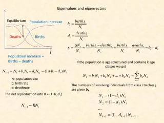
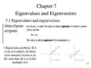
3.4 Eigenvalues and Eigenvectors Definition Let A be an n n matrix. A scalar is called an eigenvalue(特徵值,固有值)of A if there exists a nonzero vector x in Rn such that Ax = x. The vector x is called an eigenvectorcorresponding to . >0 <0 Figure 3.1
Computation of Eigenvalues and Eigenvectors Let A be an n n matrix with eigenvalue and corresponding eigenvector x. Ax = x Ax – x = 0 (A – In)x = 0 a system of linear equations, and x=0 is a solution. we need nonzero solutions many solutions |A – In| = 0 Solve |A – In| = 0 for leads to all the eigenvalues of A. On expending the determinant |A – In|, we get a polynomial in . This polynomial is called the characteristic polynomial of A. The equation |A – In| = 0 is called the characteristic equation of A.
Example 1 Find the eigenvalues and eigenvectors of the matrix Solution Find the characteristic polynomial of A: The eigenvalues of A are 2 and –1. The corresponding eigenvectors are found by using these values of in the equation(A – I2)x = 0.
(1) = 2 (A – 2I2)x = 0 Thus the eigenvectors of A corresponding to = 2 are
(2) = –1 (A + 1I2)x = 0 Thus the eigenvectors of A corresponding to = –1 are 隨堂作業:9先不求eigenspaces
Proof Let x1, x2V and let c be a scalar. Then Ax1 = x1 and Ax2 = x2. Hence, Eigenspaces Theorem 3.9 Let A be an n n matrix and an eigenvalue of A. The set V of all eigenvectors corresponding to , together with the zero vector, is a subspace of Rn. This subspace is called the eigenspace of . Thus x1+x2V. The set is closed under addition. Further, Therefore cx1 V. The set is closed under scalar multiplication. Thus V is a subspace of Rn.
Example 2 Find the eigenvalues and corresponding eigenspaces of the matrix Solution l=10 or 1
(1) = 10 Thus the eigenspace of = 10 is The set is a basis, and the dimension is 1.
(2) = 1 Thus the eigenspace of = 1 is 隨堂作業:10 If an eigenvalue occurs as a k times repeated root of the characteristic equation, we say that it is of multiplicity (重根數) k. Thus l=10 has multiplicity 1, while l=1 has multiplicity 2. The set is a basis, and the dimension is 2.