Download

1 / 53
530 likes | 649 Vues
2S 3. S 3. S 1 xS 2. From Spinning Tops to Rigid Body Motion. Peter H. Richter University of Bremen. Department of Mathematics, University of Groningen, June 3, 2009. Outline. Demonstration of some basic physics Parameter sets Configuration spaces SO(3) and S 2 vs. T 3 and T 2

E N D
2S3 S3 S1xS2 From Spinning Tops to Rigid Body Motion Peter H. RichterUniversity of Bremen Department of Mathematics, University of Groningen, June 3, 2009 Groningen, June 3, 2009
Outline • Demonstration of some basic physics • Parameter sets • Configuration spaces SO(3) and S2 vs. T3 and T2 • Phase space structure • Equations of motion • Strategies of investigation Groningen, June 3, 2009
Demonstration of some basic physics • Parameter sets • Configuration spaces SO(3) and S2 vs. T3 and T2 • Phase space structure • Equations of motion • Strategies of investigation Groningen, June 3, 2009
two moments of inertiaa, b (g = 1-a-b) two angles s,t for the center of gravity angledbetween the frame‘s axis and the direction of gravity Parameter space 6 essential parameters after scaling of lengths, time, energy: at least one independent moment of inertia r for the Cardan frame Groningen, June 3, 2009
Demonstration of some basic physics • Parameter sets • Configuration spaces SO(3) and S2 vs. T3 and T2 • Phase space structure • Equations of motion • Strategies of investigation Groningen, June 3, 2009
(j, q, y) (j + p, 2p - q, y + p) Cardan angles (j,q, y) Euler angles (j,q, y) Poisson (q, y)-sphere Poisson (q, y)-torus „polar points“ q = 0, p defined with respect to an arbitrary direction „polar y-circles“ q = 0, p defined with respect to the axes of the frame coordinate singularities removed, but Euler variables lost Configuration spaces SO(3) versus T3 after separation of angle j: reduced configuration spaces Groningen, June 3, 2009
Demonstration of some basic physics • Parameter sets • Configuration spaces SO(3) and S2 vs. T3 and T2 • Phase space structure • Equations of motion • Strategies of investigation Groningen, June 3, 2009
energy conservation h = const 5D energy surfaces strong chaos one angular momentum lz = const 4D invariant sets mild chaos 3 conserved quantities 3D invariant sets integrable 4 conserved quantities 2D invariant sets super-integrable Phase space and conserved quantities 3 angles + 3 momenta 6D phase space Groningen, June 3, 2009
energy conservation h = const 3D energy surfaces chaos integrable 2 conserved quantities 2D invariant sets super-integrable 3 conserved quantities 1D invariant sets Reduced phase spaces with parameter lz 2 angles + 2 momenta 4D phase space Groningen, June 3, 2009
energy conservation h = const 3D energy surfaces chaos 2 conserved quantities 2D invariant sets integrable 3 conserved quantities 1D invariant sets super-integrable (g,l) - phase space 3 gi-components + 3 momenta li 6D phase space 2 Casimir constants g ·g = 1 and g ·l = lz 4D simplectic space Groningen, June 3, 2009
Demonstration of some basic physics • Parameter sets • Configuration spaces SO(3) and S2 vs. T3 and T2 • Phase space structure • Equations of motion • Strategies of investigation Groningen, June 3, 2009
Coordinates: j motion: Casimir constants: Energy constant: Effective potential: Without frame: Euler-Poisson equations in (g,l)-space Groningen, June 3, 2009
where Reduction to a Hamiltonian with parameter , Coriolisforce and centrifugal potential With frame: Euler – Lagrange equations Demo Groningen, June 3, 2009
Demonstration of some basic physics • Parameter sets • Configuration spaces SO(3) and S2 vs. T3 and T2 • Phase space structure • Equations of motion • Strategies of investigation Groningen, June 3, 2009
Search for invariant sets in phase space, and their bifurcations Katok Envelope • topological bifurcations of iso-energy surfaces • their projections to configuration and momentum spaces • integrable systems: action variable representation and foliation by invariant tori • chaotic systems: Poincaré sections • periodic orbit skeleton: stable (order) and unstable (chaos) Actions Tori Poincaré Periods Groningen, June 3, 2009
1 2S3 S3 3S3 K3 RP3 7 s2 = s3 = 0 5 5 6 Katok‘s cases 1 4 1 2 3 3 2 7 colors for 7 types of bifurcation diagrams 3 6colors for 6 types of energy surfaces 7 4 5 6 S1xS2 Groningen, June 3, 2009
S3 S3 T2 2S3 2T2 T2 (1,0.6) (2.5,2.15) (h,l) = (1,1) I I‘ II 7+1 types of envelopes (I) (A1,A2,A3) = (1.7,0.9,0.86) S1xS2 M32 (2,1.8) III Groningen, June 3, 2009
RP3 K3 M32 3S3 2S2, T2 S3,S1xS2 2T2 T2 (1.85,1.705) (1.9,1.759) IV (1.5,0.6) V VI VII (1.912,1.763) 7+1 types of envelopes (II) (A1,A2,A3) = (1.7,0.9,0.86) Groningen, June 3, 2009
Energy surfaces in action representation Euler Lagrange Kovalevskaya Groningen, June 3, 2009
Examples: From Kovalevskaya to Lagrange (A1,A2,A3) = (2,,1) (s1,s2,s3) = (1,0,0) E B = 2 = 2 = 1.1 = 1.1 Groningen, June 3, 2009
Example of a bifurcation scheme of periodic orbits Groningen, June 3, 2009
Lagrange tops without frame Three types of bifurcation diagrams: 0.5 < a < 0.75 (discs), 0.75 < a < 1 (balls), a > 1 (cigars)five types of Reeb graphs When the 3-axis is the symmetry axis, the system remains integrable with the frame, otherwise not. VB Lagrange Groningen, June 3, 2009
The Katok family – and others arbitrary moments of inertia, (s1, s2, s3) = (1, 0, 0) Topology of 3D energy surfaces and 2D Poincaré surfaces of section has been analyzed completely (I. N. Gashenenko, P. H. R. 2004) How is this modified by the Cardan frame? Groningen, June 3, 2009
Invariant sets in phase space Groningen, June 3, 2009
Momentum map (h,l) bifurcation diagrams Equivalent statements: (h,l) is critical value relative equilibrium g is critical point of Ul Groningen, June 3, 2009
Rigid body dynamics in SO(3) • Phase spaces and basic equations • Full and reduced phase spaces • Euler-Poisson equations • Invariant sets and their bifurcations • Integrable cases • Euler • Lagrange • Kovalevskaya • Katok‘s more general cases • Effective potentials • Bifurcation diagrams • Enveloping surfaces • Poincaré surfaces of section • Gashenenko‘s version • Dullin-Schmidt version • An application Groningen, June 3, 2009
Lagrange: „heavy“, symmetric Kovalevskaya: A Integrable cases Euler:„gravity-free“ E L K Groningen, June 3, 2009
Poisson sphere potential admissible values in (p,q,r)-space for given l and h < Ul (h,l)-bifurcation diagram Euler‘s case l-motiondecouples from g-motion B Groningen, June 3, 2009
effective potential (p,q,r)-equations I: ½ < a < ¾ integrals bifurcation diagrams 2S3 S3 II: ¾ < a < 1 III: a > 1 S1xS2 S1xS2 RP3 RP3 S3 Lagrange‘s case Groningen, June 3, 2009
Enveloping surfaces B Groningen, June 3, 2009
(p,q,r)-equations integrals Kovalevskaya‘s case Tori projected to (p,q,r)-space Tori in phase space and Poincaré surface of section Groningen, June 3, 2009
Critical tori: additional bifurcations Fomenko representation of foliations (3 examples out of 10) „atoms“ of the Kovalevskaya system elliptic center A pitchfork bifurcation B period doubling A* double saddle C2 Groningen, June 3, 2009
Energy surfaces in action representation Euler Lagrange Kovalevskaya Groningen, June 3, 2009
Rigid body dynamics in SO(3) • Phase spaces and basic equations • Full and reduced phase spaces • Euler-Poisson equations • Invariant sets and their bifurcations • Integrable cases • Euler • Lagrange • Kovalevskaya • Katok‘s more general cases • Effective potentials • Bifurcation diagrams • Enveloping surfaces • Poincaré surfaces of section • Gashenenko‘s version • Dullin-Schmidt version • An application Groningen, June 3, 2009
2 1 2S3 S3 3S3 K3 RP3 7 s2 = s3 = 0 5 6 Katok‘s cases 1 4 3 2 7 colors for 7 types of bifurcation diagrams 3 7colors for 7 types of energy surfaces 7 4 5 6 S1xS2 Groningen, June 3, 2009
S3 3S3 l = 0 l = 1.68 l = 1.71 l = 1.74 K3 RP3 l = 1.763 l = 1.773 l = 1.86 l = 2.0 Effective potentials for case 1 (A1,A2,A3) = (1.7,0.9,0.86) Groningen, June 3, 2009
S3 S3 T2 2S3 2T2 T2 (1,0.6) (2.5,2.15) (h,l) = (1,1) I I‘ II 7+1 types of envelopes(I) (A1,A2,A3) = (1.7,0.9,0.86) S1xS2 M32 (2,1.8) III Groningen, June 3, 2009
RP3 K3 M32 3S3 2S2, T2 S3,S1xS2 2T2 T2 (1.85,1.705) (1.9,1.759) IV (1.5,0.6) V VI VII (1.912,1.763) 7+1 types of envelopes (II) (A1,A2,A3) = (1.7,0.9,0.86) Groningen, June 3, 2009
2S3 2S2 S1xS2 T2 (3.6,2.8) (3.6,2.75) III‘ II‘ 2 variations of types II and III A = (0.8,1.1,0.9) A = (0.8,1.1,1.0) Only in cases II‘ and III‘ are the envelopes free of singularities. Case II‘ occurs in Katok‘s regions 4, 6, 7, case III‘ only in region 7. This completes the list of all possible types of envelopes in the Katok case. There are more in the more general cases where only s3=0 (Gashenenko) or none of the si = 0 (not done yet). Groningen, June 3, 2009
Rigid body dynamics in SO(3) • Phase spaces and basic equations • Full and reduced phase spaces • Euler-Poisson equations • Invariant sets and their bifurcations • Integrable cases • Euler • Lagrange • Kovalevskaya • Katok‘s more general cases • Effective potentials • Bifurcation diagrams • Enveloping surfaces • Poincaré surfaces of section • Gashenenko‘s version • Dullin-Schmidt version • An application Groningen, June 3, 2009
Poincaré section S1 Skip 3 Groningen, June 3, 2009
p S+(g) S-(g) q 0 2p 2p 0 0 Poincaré section S1 – projections to S2(g) Groningen, June 3, 2009
Place the polar circles at upper and lower rims of the projection planes. Poincaré section S1 – polar circles Groningen, June 3, 2009
A =( 2, 1.1, 1) s =( 0.94868,0,0.61623) Poincaré section S1 – projection artifacts Groningen, June 3, 2009
S1: S2: where Explicit formulae for the two sections with Groningen, June 3, 2009
A =( 2, 1.1, 1) s =( 0.94868,0,0.61623) Poincaré sections S1 and S2 in comparison Groningen, June 3, 2009