Roots of Non-Linear Equations (Recap): f ( x ) = 0

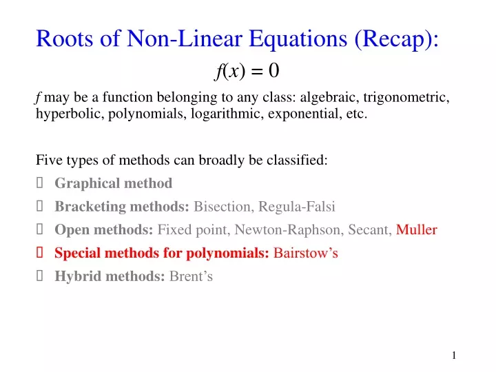
1. Roots of Non-Linear Equations (Recap): f(x) = 0 f may be a function belonging to any class: algebraic, trigonometric, hyperbolic, polynomials, logarithmic, exponential, etc. Five types of methods can broadly be classified: • Graphical method • Bracketing methods: Bisection, Regula-Falsi • Open methods: Fixed point, Newton-Raphson, Secant, Muller • Special methods for polynomials:Bairstow’s • Hybrid methods: Brent’s

2. Open Methods: Muller • Principle: fit a quadratic polynomial through three points to approximate the function. • Problem:f(x) = 0, find a root x = α such that f(α) = 0 f(x0) f(x1) f(x2) x2 x0 x1 y = f(x) x3

3. Open Methods: Muller • Initialize: choose three points x0, x1, x2 and evaluate f(x0), f(x1), f(x2). Denote f(xk) = fk • Fit a quadratic polynomial through three points xk, xk-1, xk-2 as: p(x) = a(x -xk)2 + b(x -xk) + c • Equations: p(xk) = fk = c p(xk-1) = fk-1= a(xk-1-xk)2 + b(xk-1-xk) + fk p(xk-2) = fk-2 = a(xk-2-xk)2 + b(xk-2-xk) + fk • Define Divided Differences: • 1st Divided Difference: • 2nd Divided Difference:

4. Open Methods: Muller p(xk) = fk = c …(1) p(xk-1) = fk-1= a(xk-1-xk)2 + b(xk-1-xk) + fk…(2) p(xk-2) = fk-2 = a(xk-2-xk)2 + b(xk-2-xk) + fk…(3) • Rearrange (2) and (3) as: • Dividing both sides by and , respectively, and rearranging:

5. Open Methods: Muller = • Express LHS in terms of Newton’s Divided Differences: • Solutions (eqs. (4) – (5)): =

6. Properties of Divided Differences 2nd Divided Difference:

7. Note: Properties of Divided Differences • 1st Divided Difference: • 2nd Divided Difference: We shall use these properties for the Theory of Approximation!

8. Open Methods: Muller • Principle: fit a quadratic polynomial through three points to approximate the function. • Problem:f(x) = 0, find a root x = α such that f(α) = 0 • Initialize: choose three points x0, x1, x2 and evaluate f(x0), f(x1), f(x2) • Fit a quadratic polynomial through three points xk, xk-1, xk-2 as: p(x) = a(x -xk)2 + b(x -xk) + c • Constants: c =f(xk); b = f[xk, xk-1] + (xk- xk-1)f[xk, xk-1, xk-2]; a = f[xk, xk-1, xk-2] • Iteration step k: or • Stopping criteria:

9. Tutorial 2 Problem 2: Muller • 2. Find a root of the following equation using Muller’s method to an approximate error of : • Take three starting values as 1, 2 and 3 in the Muller’s method. Do they converge to the same root as the Secant Method? Compare the number of iterations required in two methods. Prob 2_Tut2.xls

10. Open Methods: Muller • Convergence: Analysis is similar to Secant method, using Newton’s Polynomial. as , = constant

11. Order of Convergence • Definition: Let be a sequence which converges to α. Define en = xn – α. If there exists a number p and a constant C ≠ 0 such that, Then, p is called the order of convergence of the sequence and C is the asymptotic error constant. • Fixed Point: = C, 1st Order. • Newton Raphson: = C, 2nd Order • Secant: = C, mixed order, ≈ 1.6 • Muller: = C, mixed order, ≈ 1.84

12. Polynomial Methods: Single Root If we divide by a factor (x - r) such that, r = α is a root of the polynomial, we will get an exact polynomial of order (n - 1). If r ≠ α, dividing by a factor (x - r) will have a remainder b0.

13. Polynomial Methods: Single Root

14. Polynomial Methods: Single Root b0 is a function of r → b0(r), at r = α, b0(r) = 0 Problem:f(x) = 0, find a root x = α such that f(α) = 0 Problem:b0(r) = 0, find a root r = α such that b0(α) = 0 Apply Newton-Raphson: Iteration Formula for Step k: or → b0’(r) = b1 → Assume a value of r, estimate b0 and b1, compute new r. Continue until b0 becomes zero. (with acceptable relative error)

15. Polynomial Methods: Bairstow Let us divide by a factor (x2– rx – s). If the factor is exact, the resulting polynomial will be of order (n – 2). Two roots of the polynomial can be estimated simultaneously as the roots of the quadratic factor. For the complex roots, they will be the complex conjugates. If the factor (x2– rx – s) is not exact, there will be two remainder terms, one function of x and another constant. Let us express the remainder term as b1(x - r) + b0. This form instead of the standard b1x + b0 is chosen to device a convenient iteration formula!

16. Polynomial Methods: Bairstow

17. Polynomial Methods: Bairstow b0 and b1 are functions of r and s → b0(r, s) and b1(r, s) Expand in Taylor’s series: Apply 2-d Newton-Raphson Need to evaluate: , , and

18. Polynomial Methods: Bairstow Partial differentials with respect to r:

19. Polynomial Methods: Bairstow Partial differentials with respect to s:

20. Polynomial Methods: Bairstow ; ; and For any given polynomial, we know {a0, a1, … an}. Assume r and s. Compute {b0, b1, … bn} and {c0, c1, … cn}. Compute Δr and Δs.

21. Polynomial Methods: Bairstow Algorithm • Step 1: input a0, a1, … an and initialize r and s. • Step 2: compute b0, b1, … bn • Step 3: compute c0, c1, … cn • Step 4: compute Δr and Δs from • Step 5: compute rnew = r + Δr, snew = s + Δs • Step 6: check for convergence, and b0, b1 ≤ εʹ • Step 7: Stop if all convergence checks are satisfied. Else, set r = rnew, s = snew and go to step 2.

22. Multiple Roots • Definition: A root α of the equation f(x) = 0 is said to have a multiplicity of q if, when, q > 1, the order of convergence are no longer valid. • Solution: Suppose a function f(x) is q-times continuously differentiable in the neighbourhood of a root α of multiplicity q, and where Define Therefore,α is a root of f(x) of multiplicity q but is a simple root of u(x)!