Download
1 / 53
530 likes | 749 Vues
Minimizing Communication in Numerical Linear Algebra www.cs.berkeley.edu/~demmel Optimizing One-sided Factorizations: LU and QR. Jim Demmel EECS & Math Departments, UC Berkeley demmel@cs.berkeley.edu. Outline. Recall results for Matmul from last time

E N D
Minimizing Communication in Numerical Linear Algebrawww.cs.berkeley.edu/~demmelOptimizing One-sided Factorizations: LU and QR Jim Demmel EECS & Math Departments, UC Berkeley demmel@cs.berkeley.edu
Outline • Recall results for Matmul from last time • Review Gaussian Elimination (GE) for solving Ax=b • Optimizing GE for caches on sequential machines • using matrix-matrix multiplication (BLAS and LAPACK) • Minimizing communication for sequential GE • Not LAPACK, but Recursive LU minimizes bandwidth (not latency) • Data layouts on parallel machines • Parallel Gaussian Elimination (ScaLAPACK) • Minimizing communication for parallel GE • Not ScaLAPACK, but “Comm-Avoiding LU” (CALU) • Same idea for minimizing bandwidth and latency in sequential case • Ditto for QR Summer School Lecture 4
Summary of Matrix Multiplication • Goal: Multiply n x n matrices C = A·B using O(n3) arithmetic operations, minimizing data movement • Sequential • Assume fast memory of size M < 3n2, count slow mem. refs. • Thm: need (n3/M1/2) slow mem. refs. and (n3/M3/2) messages • Attainable using “blocked matrix multiply” • Parallel • Assume P processors, O(n2/P) data per processor • Thm: need (n2/P1/2) words sent and (P1/2) messages • Attainable by Cannon, nearly by SUMMA • SUMMA used in practice (PBLAS) • Which other linear algebra problems can we do with as little data movement? • Today: A=PLU, A=QR in detail, summarize what’s known, open Summer School Lecture 4
Sca/LAPACK Overview Summer School Lecture 4
Gaussian Elimination (GE) for solving Ax=b • Add multiples of each row to later rows to make A upper triangular • Solve resulting triangular system Ux = c by substitution … for each column i … zero it out below the diagonal by adding multiples of row i to later rows for i = 1 to n-1 … for each row j below row i for j = i+1 to n … add a multiple of row i to row j tmp = A(j,i); for k = i to n A(j,k) = A(j,k) - (tmp/A(i,i)) * A(i,k) … 0 . . . 0 0 . . . 0 0 . . . 0 0 . . . 0 0 . . . 0 0 . . . 0 0 . . . 0 0 . 0 0 . 0 0 0 0 After i=1 After i=2 After i=3 After i=n-1 Summer School Lecture 4
Refine GE Algorithm (1/5) • Initial Version • Remove computation of constant tmp/A(i,i) from inner loop. … for each column i … zero it out below the diagonal by adding multiples of row i to later rows for i = 1 to n-1 … for each row j below row i for j = i+1 to n … add a multiple of row i to row j tmp = A(j,i); for k = i to n A(j,k) = A(j,k) - (tmp/A(i,i)) * A(i,k) for i = 1 to n-1 for j = i+1 to n m = A(j,i)/A(i,i) for k = i to n A(j,k) = A(j,k) - m * A(i,k) i m j Summer School Lecture 4
Refine GE Algorithm (2/5) • Last version • Don’t compute what we already know: zeros below diagonal in column i for i = 1 to n-1 for j = i+1 to n m = A(j,i)/A(i,i) for k = i to n A(j,k) = A(j,k) - m * A(i,k) for i = 1 to n-1 for j = i+1 to n m = A(j,i)/A(i,i) for k = i+1 to n A(j,k) = A(j,k) - m * A(i,k) i m j Do not compute zeros Summer School Lecture 4
Refine GE Algorithm (3/5) • Last version • Store multipliers m below diagonal in zeroed entries for later use for i = 1 to n-1 for j = i+1 to n m = A(j,i)/A(i,i) for k = i+1 to n A(j,k) = A(j,k) - m * A(i,k) for i = 1 to n-1 for j = i+1 to n A(j,i) = A(j,i)/A(i,i) for k = i+1 to n A(j,k) = A(j,k) - A(j,i) * A(i,k) i m j Store m here Summer School Lecture 4
Refine GE Algorithm (4/5) • Last version for i = 1 to n-1 for j = i+1 to n A(j,i) = A(j,i)/A(i,i) for k = i+1 to n A(j,k) = A(j,k) - A(j,i) * A(i,k) • Split Loop for i = 1 to n-1 for j = i+1 to n A(j,i) = A(j,i)/A(i,i) for j = i+1 to n for k = i+1 to n A(j,k) = A(j,k) - A(j,i) * A(i,k) i j Store all m’s here before updating rest of matrix Summer School Lecture 4
Refine GE Algorithm (5/5) for i = 1 to n-1 for j = i+1 to n A(j,i) = A(j,i)/A(i,i) for j = i+1 to n for k = i+1 to n A(j,k) = A(j,k) - A(j,i) * A(i,k) • Last version • Express using matrix operations (BLAS) for i = 1 to n-1 A(i+1:n,i) = A(i+1:n,i) * ( 1 / A(i,i) ) … BLAS 1 (scale a vector) A(i+1:n,i+1:n) = A(i+1:n , i+1:n ) - A(i+1:n , i) * A(i , i+1:n) … BLAS 2 (rank-1 update) Summer School Lecture 4
What GE really computes for i = 1 to n-1 A(i+1:n,i) = A(i+1:n,i) / A(i,i) … BLAS 1 (scale a vector) A(i+1:n,i+1:n) = A(i+1:n , i+1:n ) - A(i+1:n , i) * A(i , i+1:n) … BLAS 2 (rank-1 update) • Call the strictly lower triangular matrix of multipliers M, and let L = I+M • Call the upper triangle of the final matrix U • Lemma (LU Factorization): If the above algorithm terminates (does not divide by zero) then A = L*U • Solving A*x=b using GE • Factorize A = L*U using GE (cost = 2/3 n3 flops) • Solve L*y = b for y, using substitution (cost = n2 flops) • Solve U*x = y for x, using substitution (cost = n2 flops) • Thus A*x = (L*U)*x = L*(U*x) = L*y = b as desired Summer School Lecture 4
Problems with basic GE algorithm for i = 1 to n-1 A(i+1:n,i) = A(i+1:n,i) / A(i,i) … BLAS 1 (scale a vector) A(i+1:n,i+1:n) = A(i+1:n , i+1:n ) … BLAS 2 (rank-1 update) - A(i+1:n , i) * A(i , i+1:n) • What if some A(i,i) is zero? Or very small? • Result may not exist, or be “unstable”, so need to pivot • Current computation all BLAS 1 or BLAS 2, but we know that BLAS 3 (matrix multiply) is fastest (earlier lectures…) Peak BLAS 3 BLAS 2 BLAS 1 Summer School Lecture 4
Pivoting in Gaussian Elimination • A = [ 0 1 ] fails completely because can’t divide by A(1,1)=0 • [ 1 0 ] • But solving Ax=b should be easy! • When diagonal A(i,i) is tiny (not just zero), algorithm may terminate but get completely wrong answer • Numerical instability • Roundoff error is cause • Cure:Pivot (swap rows of A) so A(i,i) large • Conventional pivoting: Partial Pivoting (GEPP) • Not compatible with minimizing latency (apparently!), but we will start with it… Summer School Lecture 4
Gaussian Elimination with Partial Pivoting (GEPP) • Partial Pivoting: swap rows so that A(i,i) is largest in column for i = 1 to n-1 find and record k where |A(k,i)| = max{i j n} |A(j,i)| … i.e. largest entry in rest of column i if |A(k,i)| = 0 exit with a warning that A is singular, or nearly so elseif k ≠ i swap rows i and k of A end if A(i+1:n,i) = A(i+1:n,i) / A(i,i) … each |quotient| ≤ 1 A(i+1:n,i+1:n) = A(i+1:n , i+1:n ) - A(i+1:n , i) * A(i , i+1:n) • Lemma: This algorithm computes A = P*L*U, where P is a permutation matrix. • This algorithm is numerically stable in practice • For details see LAPACK code at • http://www.netlib.org/lapack/single/sgetf2.f • Standard approach – but communication costs? Summer School Lecture 4
Problems with basic GE algorithm • What if some A(i,i) is zero? Or very small? • Result may not exist, or be “unstable”, so need to pivot • Current computation all BLAS 1 or BLAS 2, but we know that BLAS 3 (matrix multiply) is fastest (earlier lectures…) for i = 1 to n-1 A(i+1:n,i) = A(i+1:n,i) / A(i,i) … BLAS 1 (scale a vector) A(i+1:n,i+1:n) = A(i+1:n , i+1:n ) … BLAS 2 (rank-1 update) - A(i+1:n , i) * A(i , i+1:n) Peak BLAS 3 BLAS 2 BLAS 1 Summer School Lecture 4
Converting BLAS2 to BLAS3 in GEPP • Blocking • Used to optimize matrix-multiplication • Harder here because of data dependencies in GEPP • BIG IDEA: Delayed Updates • Save updates to “trailing matrix” from several consecutive BLAS2 (rank-1) updates • Apply many updates simultaneously in one BLAS3 (matmul) operation • Same idea works for much of dense linear algebra • One-sided factorization are ~100% BLAS3 • Two-sided factorizations are ~50% BLAS3 • First Approach: Need to choose a block size b • Algorithm will save and apply b updates • b should be small enough so that active submatrix consisting of b columns of A fits in cache • b should be large enough to make BLAS3 (matmul) fast Summer School Lecture 4
Blocked GEPP (www.netlib.org/lapack/single/sgetrf.f) for ib = 1 to n-1 step b … Process matrix b columns at a time end = ib + b-1 … Point to end of block of b columns apply BLAS2 version of GEPP to get A(ib:n , ib:end) = P’ * L’ * U’ … let LL denote the strict lower triangular part of A(ib:end , ib:end) + I A(ib:end , end+1:n) = LL-1 * A(ib:end , end+1:n)… update next b rows of U A(end+1:n , end+1:n ) = A(end+1:n , end+1:n ) - A(end+1:n , ib:end) * A(ib:end , end+1:n) … apply delayed updates with single matrix-multiply … with inner dimension b (For a correctness proof, see on-line notes from CS267 / 1996.) CS267 Lecture 9
Efficiency of Blocked GEPP (all parallelism “hidden” inside the BLAS) Summer School Lecture 4
Blocked QR decomposition • Same blocked decomposition idea as for LU works for QR • However, need to some extra work to apply sequence of “column eliminations” = Householder transformations • j=1 to b (I – j·uj·uTj ) = I – U·T· UT where • Each I – ·u·uT is orthogonal • Conventionally: = 2 / uT·u • Latest LAPACK release does it differently … • U = [ u1 , … , ub ] • T is b x b and triangular Summer School Lecture 4
Communication Lower Bound for GE I 0 -B I I 0 -B A I 0 = A I · I A·B 0 0 I 0 0 I I • Homework: Can you use this approach for Cholesky? • A different proof than before, just for GE • If we know matmul is “hard”, can we show GE is at least as hard? • Approach: “Reduce” matmul to GE • Not a good way to do matmul but it shows that GE needs at least as much communication as matmul Summer School Lecture 4
Does GE Minimize Communication? (1/4) for ib = 1 to n-1 step b … Process matrix b columns at a time end = ib + b-1 … Point to end of block of b columns apply BLAS2 version of GEPP to get A(ib:n , ib:end) = P’ * L’ * U’ … let LL denote the strict lower triangular part of A(ib:end , ib:end) + I A(ib:end , end+1:n) = LL-1 * A(ib:end , end+1:n)… update next b rows of U A(end+1:n , end+1:n ) = A(end+1:n , end+1:n ) - A(end+1:n , ib:end) * A(ib:end , end+1:n) … apply delayed updates with single matrix-multiply … with inner dimension b • Model of communication costs with fast memory M • BLAS2 version of GEPP costs • O(n ·b) if panel fits in M: n·b M • O(n · b2) (#flops) if panel does not fit in M: n·b > M • Update of A(end+1:n , end+1:n ) by matmul costs • O( max ( n·b·n / M1/2 , n2 )) • Triangular solve with LL bounded by above term • Total # slow mem refs for GE = (n/b) · sum of above terms Summer School Lecture 4
Does GE Minimize Communication? (2/4) • Model of communication costs with fast memory M • BLAS2 version of GEPP costs • O(n ·b) if panel fits in M: n·b M • O(n · b2) (#flops) if panel does not fit in M: n·b > M • Update of A(end+1:n , end+1:n ) by matmul costs • O( max ( n·b·n / M1/2 , n2 )) • Triangular solve with LL bounded by above term • Total # slow mem refs for GE = (n/b) · sum of above terms • Case 1: M < n (one column too large for fast mem) • Total # slow mem refs for GE = (n/b)*O(max(n b2 , b n2 / M1/2 , n2 )) = O( max( n2 b , n3/ M1/2 , n3 / b )) • Minimize by choosing b = M1/2 • Get desired lower bound O(n3 / M1/2 ) Summer School Lecture 4
Does GE Minimize Communication? (3/4) • Model of communication costs with fast memory M • BLAS2 version of GEPP costs • O(n ·b) if panel fits in M: n·b M • O(n · b2) (#flops) if panel does not fit in M: n·b > M • Update of A(end+1:n , end+1:n ) by matmul costs • O( max ( n·b·n / M1/2 , n2 )) • Triangular solve with LL bounded by above term • Total # slow mem refs for GE = (n/b) · sum of above terms • Case 2: M2/3 < n M • Total # slow mem refs for GE = (n/b)*O(max(n b2 , b n2 / M1/2 , n2 )) = O( max( n2 b , n3/ M1/2 , n3 / b )) • Minimize by choosing b = n1/2 (panel does not fit in M) • Get O(n2.5) slow mem refs • Exceeds lower bound O(n3 / M1/2) by factor (M/n)1/2 M1/6 Summer School Lecture 4
Does GE Minimize Communication? (4/4) • Model of communication costs with fast memory M • BLAS2 version of GEPP costs • O(n ·b) if panel fits in M: n·b M • O(n · b2) (#flops) if panel does not fit in M: n·b > M • Update of A(end+1:n , end+1:n ) by matmul costs • O( max ( n·b·n / M1/2 , n2 )) • Triangular solve with LL bounded by above term • Total # slow mem refs for GE = (n/b) · sum of above terms • Case 3: M1/2 < n M2/3 • Total # slow mem refs for GE = (n/b)*O(max(n b, b n2 / M1/2 , n2 )) = O(max( n2 , n3/ M1/2 , n3 / b )) • Minimize by choosing b = M/n (panel fits in M) • Get O(n4/M) slow mem refs • Exceeds lower bound O(n3 / M1/2) by factor n/M1/2 M1/6 • Case 4: n M1/2 – whole matrix fits in fast mem
Homework Check omitted details in previous analysis of conventional GE Summer School Lecture 4
Alternative cache-oblivious GE formulation (1/2) A = L * U function [L,U] = RLU (A) … assume A is m by n if (n=1) L = A/A(1,1), U = A(1,1) else [L1,U1] = RLU( A(1:m , 1:n/2)) … do left half of A … let L11 denote top n/2 rows of L1 A( 1:n/2 , n/2+1 : n ) = L11-1 * A( 1:n/2 , n/2+1 : n ) … update top n/2 rows of right half of A A( n/2+1: m, n/2+1:n ) = A( n/2+1: m, n/2+1:n ) - A( n/2+1: m, 1:n/2 ) * A( 1:n/2 , n/2+1 : n ) … update rest of right half of A [L2,U2] = RLU( A(n/2+1:m , n/2+1:n) ) … do right half of A return [ L1,[0;L2] ] and [U1,[ A(.,.) ; U2 ] ] • Toledo (1997) • Describe without pivoting for simplicity • “Do left half of matrix, then right half” Summer School Lecture 4
Alternative cache-oblivious GE formulation (2/2) function [L,U] = RLU (A) … assume A is m by n if (n=1) L = A/A(1,1), U = A(1,1) else [L1,U1] = RLU( A(1:m , 1:n/2)) … do left half of A … let L11 denote top n/2 rows of L1 A( 1:n/2 , n/2+1 : n ) = L11-1 * A( 1:n/2 , n/2+1 : n ) … update top n/2 rows of right half of A A( n/2+1: m, n/2+1:n ) = A( n/2+1: m, n/2+1:n ) - A( n/2+1: m, 1:n/2 ) * A( 1:n/2 , n/2+1 : n ) … update rest of right half of A [L2,U2] = RLU( A(n/2+1:m , n/2+1:n) ) … do right half of A return [ L1,[0;L2] ] and [U1,[ A(.,.) ; U2 ] ] • Mem(m,n) = Mem(m,n/2) + O(max(m·n,m·n2/M1/2)) + Mem(m-n/2,n/2) 2 · Mem(m,n/2) + O(max(m·n,m·n2/M1/2)) = O(m·n2/M1/2 + m·n·log M) = O(m·n2/M1/2 ) if M1/2·log M = O(n)
Homework • Same recursive approach works for QR • Try it in Matlab • Hint: Elmroth / Gustavson Summer School Lecture 4
What about latency? • Neither formulation minimizes it • Two reasons: • Need a different data structure • Need a different pivoting scheme (that’s still stable!) • More later Summer School Lecture 4
Explicitly Parallelizing Gaussian Elimination • Parallelization steps • Decomposition: identify enough parallel work, but not too much • Assignment: load balance work among threads • Orchestrate: communication and synchronization • Mapping: which processors execute which threads (locality) • Decomposition • In BLAS 2 algorithm nearly each flop in inner loop can be done in parallel, so with n2 processors, need 3n parallel steps, O(n log n) with pivoting • This is too fine-grained, prefer calls to local matmuls instead • Need to use parallel matrix multiplication • Assignment and Mapping • Which processors are responsible for which submatrices? for i = 1 to n-1 A(i+1:n,i) = A(i+1:n,i) / A(i,i) … BLAS 1 (scale a vector) A(i+1:n,i+1:n) = A(i+1:n , i+1:n ) … BLAS 2 (rank-1 update) - A(i+1:n , i) * A(i , i+1:n) Summer School Lecture 4
Different Data Layouts for Parallel GE Bad load balance: P0 idle after first n/4 steps Load balanced, but can’t easily use BLAS2 or BLAS3 1) 1D Column Blocked Layout 2) 1D Column Cyclic Layout Can trade load balance and BLAS2/3 performance by choosing b, but factorization of block column is a bottleneck Complicated addressing, May not want full parallelism In each column, row b 4) Block Skewed Layout 3) 1D Column Block Cyclic Layout Bad load balance: P0 idle after first n/2 steps The winner! 6) 2D Row and Column Block Cyclic Layout 5) 2D Row and Column Blocked Layout Summer School Lecture 4
Distributed GE with a 2D Block Cyclic Layout CS267 Lecture 9
Matrix multiply of green = green - blue * pink CS267 Lecture 9
Review of Parallel MatMul • Want Large Problem Size Per Processor • PDGEMM = PBLAS matrix multiply • Observations: • For fixed N, as P increasesn Mflops increases, but less than 100% efficiency • For fixed P, as N increases, Mflops (efficiency) rises • DGEMM = BLAS routine • for matrix multiply • Maximum speed for PDGEMM • = # Procs * speed of DGEMM • Observations: • Efficiency always at least 48% • For fixed N, as P increases, efficiency drops • For fixed P, as N increases, efficiency increases CS267 Lecture 14
PDGESV = ScaLAPACK Parallel LU • Since it can run no faster than its • inner loop (PDGEMM), we measure: • Efficiency = • Speed(PDGESV)/Speed(PDGEMM) • Observations: • Efficiency well above 50% for large enough problems • For fixed N, as P increases, efficiency decreases (just as for PDGEMM) • For fixed P, as N increases efficiency increases (just as for PDGEMM) • From bottom table, cost of solving • Ax=b about half of matrix multiply for large enough matrices. • From the flop counts we would expect it to be (2*n3)/(2/3*n3) = 3 times faster, but communication makes it a little slower. CS267 Lecture 14
Does ScaLAPACK Minimize Communication? • Lower Bound: O(n2 / P1/2 ) words sent in O(P1/2 ) mess. • Attained by Cannon for matmul • ScaLAPACK: • O(n2 log P / P1/2 ) words sent – close enough • O(n log P ) messages – too large • Why so many? One reduction (costs O(log P)) per column to find maximum pivot • Need to abandon partial pivoting to reduce #messages • Let’s look at QR first, which has an analogous obstacle • one reduction per column to get its norm • Suppose we have n x n matrix on P1/2 x P1/2 processor grid • Goal: For each panel of b columns spread over P1/2 procs, identify b “good” pivot rows in one reduction • Call this factorization TSLU = “Tall Skinny LU” • Several natural bad (numerically unstable) ways explored, but good way exists • SC08, “Communication Avoiding GE”, D., Grigori, Xiang Summer School Lecture 4
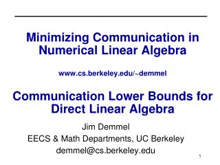
QR of a tall, skinny matrix is bottleneck;Use TSQR instead: example using 4 procs Q is represented implicitly as a product (tree of factors) [DGHL08]
Minimizing Communication in TSQR R00 R10 R20 R30 W0 W1 W2 W3 R01 Parallel: W = R02 R11 R00 W0 W1 W2 W3 Sequential: R01 W = R02 R03 R00 R01 W0 W1 W2 W3 R01 Dual Core: W = R02 R11 R03 R11 Multicore / Multisocket / Multirack / Multisite / Out-of-core: ? Can Choose reduction tree dynamically
Performance of TSQR vs Sca/LAPACK • Parallel • Intel Clovertown • Up to 8x speedup (8 core, dual socket, 10M x 10) • Pentium III cluster, Dolphin Interconnect, MPICH • Up to 6.7x speedup (16 procs, 100K x 200) • BlueGene/L • Up to 4x speedup (32 procs, 1M x 50) • All use Elmroth-Gustavson locally – enabled by TSQR • Tesla – early results (work in progress) • Up to 2.5x speedup (vs LAPACK on Nehalem) • Better: 10x on Fermi with standard algorithm and better SGEMV • Sequential • OOC on PowerPC laptop • As little as 2x slowdown vs (predicted) infinite DRAM • LAPACK with virtual memory never finished • Grid – 4x on 4 cities (Dongarra et al) • Cloud – early result – up and running using Nexus • See UC Berkeley EECS Tech Report 2008-89 • General CAQR = Communication-Avoiding QR in progress
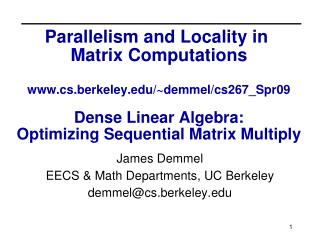
Modeled Speedups of CAQR vs ScaLAPACK Petascale up to 22.9x IBM Power 5 up to 9.7x “Grid” up to 11x Petascale machine with 8192 procs, each at 500 GFlops/s, a bandwidth of 4 GB/s.
Summary of dense sequential QR algorithms attaining communication lower bounds • Algorithms shown minimizing # Messages assume (recursive) block layout • Many references (see reports), only some shown, plus ours • Oldest reference may or may not include analysis • Cache-oblivious are underlined, Green are ours, ? is unknown/future work • b = block size, M = fast memory size, n = dimension
Back to LU: Using similar idea for TSLU as TSQR: Use reduction tree, to do “Tournament Pivoting” W1 W2 W3 W4 W1’ W2’ W3’ W4’ P1·L1·U1 P2·L2·U2 P3·L3·U3 P4·L4·U4 Choose b pivot rows of W1, call them W1’ Choose b pivot rows of W2, call them W2’ Choose b pivot rows of W3, call them W3’ Choose b pivot rows of W4, call them W4’ Wnxb = = Choose b pivot rows, call them W12’ Choose b pivot rows, call them W34’ = P12·L12·U12 P34·L34·U34 = P1234·L1234·U1234 Choose b pivot rows W12’ W34’ Go back to W and use these b pivot rows (move them to top, do LU without pivoting) Summer School Lecture 4
Minimizing Communication in TSLU LU LU LU LU W1 W2 W3 W4 LU Parallel: (binary tree) W = LU LU LU W1 W2 W3 W4 Sequential: (flat tree) LU W = LU LU LU LU W1 W2 W3 W4 LU Dual Core: W = LU LU LU LU Multicore / Multisocket / Multirack / Multisite / Out-of-core: Can Choose reduction tree dynamically, as before Summer School Lecture 4
Making TSLU Numerically Stable • Stability Goal: Make ||A – PLU|| very small: O(machine_epsilon · ||A||) • Details matter • Going up the tree, we could do LU either on original rows of W (tournament pivoting), or computed rows of U • Only tournament pivoting stable • Thm: New scheme as stable as Partial Pivoting (PP) in following sense: get same results as PP applied to different input matrix whose entries are blocks taken from input A • CALU – Communication Avoiding LU for general A • Use TSLU for panel factorizations • Apply to rest of matrix • Cost: redundant panel factorizations (extra O(n2) flops – ok) • Benefit: • Stable in practice, but not same pivot choice as GEPP • One reduction operation per panel: reduces latency to minimum Summer School Lecture 4
Sketch of TSLU Stabilty Proof A11 A21 A31 A’11 · = = · U’11 U’12 As22 As32 U’11 U’12 U21 -L21-1 ·A21· U’11-1· U’12 As32 A11 A12 A21 A22 A31 A32 A11 A12 A21 A22 A31 A32 A’11 A’12 A’21 A’22 A31 A32 L’11 L’21I L’31 0 I A’11 A’12 A21 A21 -A31 A32 L’11 A21·U’11-1 L21 -L31 I 11 12 0 2122 0 0 0 I A21 G = = · Need to show As32 same as above • Consider A = with TSLU of first columns done by : (assume wlog that A21 already contains desired pivot rows) • Resulting LU decomposition (first n/2 steps) is • Claim: As32 can be obtained by GEPP on larger matrix formed from blocks of A • GEPP applied to G pivots no rows, and L31 · L21-1 ·A21· U’11-1· U’12+As32= L31 · U21 · U’11-1· U’12+As32 = A31· U’11-1· U’12+As32 = L’31· U’12+As32= A32 Summer School Lecture 4
Stability of LU using TSLU: CALU (1/2) • Worst case analysis • Pivot growth factor from one panel factorization with b columns • TSLU: • Proven: 2bH where H = 1 + height of reduction tree • Attained: 2b, same as GEPP • Pivot growth factor on m x n matrix • TSLU: • Proven: 2nH-1 • Attained: 2n-1, same as GEPP • |L| can be as large as 2(b-2)H-b+1 , but CALU still stable • There are examples where GEPP is exponentially less stable than CALU, and vice-versa, so neither is always better than the other • Discovered sparse matrices with O(2n) pivot growth Summer School Lecture 4
Stability of LU using TSLU: CALU (2/2) • Empirical testing • Both random matrices and “special ones” • Both binary tree (BCALU) and flat-tree (FCALU) • 3 metrics: ||PA-LU||/||A||, normwise and componentwise backward errors • See [D., Grigori, Xiang, 2010] for details Summer School Lecture 4
Performance vs ScaLAPACK • TSLU • IBM Power 5 • Up to 4.37x faster (16 procs, 1M x 150) • Cray XT4 • Up to 5.52x faster (8 procs, 1M x 150) • CALU • IBM Power 5 • Up to 2.29x faster (64 procs, 1000 x 1000) • Cray XT4 • Up to 1.81x faster (64 procs, 1000 x 1000) • See INRIA Tech Report 6523 (2008), paper at SC08 Summer School Lecture 4
CALU speedup prediction for a Petascale machine - up to 81x faster P = 8192 Petascale machine with 8192 procs, each at 500 GFlops/s, a bandwidth of 4 GB/s.
Summary of dense sequential LU algorithms attaining communication lower bounds • Algorithms shown minimizing # Messages assume (recursive) block layout • Many references (see reports), only some shown, plus ours • Oldest reference may or may not include analysis • Cache-oblivious are underlined, Green are ours, ? is unknown/future work • b = block size, M = fast memory size, n = dimension
![Modeling MEMS Sensors [SUGAR: A Computer Aided Design Tool for MEMS ]](https://cdn1.slideserve.com/3083615/modeling-mems-sensors-sugar-a-computer-aided-design-tool-for-mems-dt.jpg)