Download

1 / 22
220 likes | 380 Vues
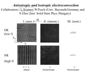
Anisotropic and isotropic electroconvection. Collaborators: L.Kramer, W.Pesch (Univ. Bayreuth/Germany and N.Eber (Inst. Solid State Phys./Hungary). H. I. (anis.). II. (interm.). III. (isotr.). OR (low f). y. x. NR (high f). +. +. planar. homeotropic.

E N D
Anisotropic and isotropic electroconvection Collaborators: L.Kramer, W.Pesch (Univ. Bayreuth/Germany and N.Eber (Inst. Solid State Phys./Hungary) H I. (anis.) II. (interm.) III. (isotr.) OR (low f) y x NR (high f) + + planar homeotropic homeotropic
ELECTROHYDRODYNAMICS OF NEMATICS STANDARD - free energy density - balance of torques - equation of motion - incompressibility - equation of electrostatics -charge conservation MODEL (SM)
Material parameters: Boundary conditions: planar or homeotropic Relevant: alignment + sign of a and a 8 combinations planar, a < 0, a > 0 anisotropic homeotropic,a < 0, a > 0 intermediate homeotropic, a > 0, a < 0isotropic IV. planar, a < 0, a < 0non-standard SM
I. planar, a < 0, a > 0 anisotropic Ginzburg-Landau description works MBBA: - 0.13
At threshold, increasing f (planar, a > 0, a < 0): OR NR n TW (non-stand.) DR
H drives between semi-isotropic and anisotropic • soft <-> patterning mode • direct transition to STC • AR-s • chevron formation • defect glide • 2 LP-s NR OR
Homeotropic alignment (standard, semi-isotropic) (A.Rossberg, L.Kramer) OR NR theor. exp.
III. Homeotropic, a > 0, a < 0 ( truly isotropic) Direct transition to isotropic EC
Swift-Hohenberg eq. (W.Pesch, L.Kramer, B.Dressel) At onset: exp. theo. f nonlinear regime: hard squares soft squares : not reproduced
IV. planar, a < 0, a < 0: no standard pattern (conductive)
PR or oblique • nz= 0, no shadowgraph • ny (?) oscillates • Uc~ d, f • - qc is d indep. Experimental: Dielectric mode! (LK)
I and II- conductive III and IV - dielectric
1. Dielectric mode for MBBA (planar, a < 0, a > 0) 2. Dielectric mode for MBBA (planar, a < 0, a < 0) - no pattern Flexoelectricity
Flexoelectricity Effect on the roll angle, only for d.c. (only in conductive)
3. Dielectric mode for MBBA (planar, a < 0, a < 0) + flexoelectricity e1- e3= 1.34 e1+ e3= -7.84 finite threshold! obliqueness!
4. Dielectric mode for MBBA (planar, a < 0, a < 0) + flexoelectricity e1- e3= 2.68 e1+ e3= -7.84 (A.Krekhov, W.Pesch)
planar, a < 0, a < 0: no standard pattern (conductive) • dielectric mode at low f • SM + flexoelectricity • why is DM more sensitive to flexo, than CM?