Transparency

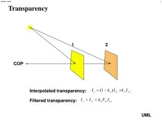
1. Transparency 1 2 COP Interpolated transparency: Filtered transparency:

2. Alpha Blending can be thought of as transparency. (R, G, B, A) Source and destination factors: Source Destination Projection Plane Frame Buffer

3. Alpha Blending Enabling: glEnable(GL_BLEND); Setting up factors: glBlendFunc(sfactor, dfactor); Factor choices: GL_ZERO (0,0,0,0) GL_ONE (1,1,1,1) GL_DST_COLOR GL_SRC_COLOR GL_ONE_MINUS_DST_COLOR (1,1,1,1)- GL_ONE_MINUS_SRC_COLOR (1,1,1,1)- GL_SRC_ALPHA GL_ONE_MINUS_SRC_ALPHA (1,1,1,1)- GL_DST_ALPHA GL_ONE_MINUS_DST_ALPHA (1,1,1,1)-

4. Refractive Transparency n Snell’s Law: -n

5. Implementation Strategies in Graphics Object oriented: for(each_object) render (object); - Pipelined vertex oriented renderer fits this strategy - Any primitive potentially affects any set of pixels in the frame buffer/z buffer - Usually implemented in hardware Image oriented: for (each_pixel) assign_a_color (pixel); - Requires limited display memory - Can exploit coherence in incremental algorithms - Requires complex geometric data structure

6. Ray Tracing • Descartes, 1637 • Whitted, 1980 • Integrates aspects of rendering handled separately in the object/pipeline approach • Hidden surface (Z-buffer) • Reflections (Transformation and stencil techniques) • Shadows (Projection, shadow buffer, shadow map) • Adds the ability to handle refraction through transparent/translucent objects • Adds the ability to handle global specular interactions • Computationally costly: not a real-time rendering method • The realism is striking, but unreal • Most useful in combination with or to augment other techniques

7. Visible Surface Ray Tracing p2 p1 COP for (each pixel in projection plane){ construct ray from center of projection through pixel for (each object in scene) if (object is intersected by ray) and (intersection is closest so far) record intersection point and object id; for (each light) determine pixel color using lighting equation at intersection point }

8. At the Ray Intersection: Light Source l Object Intersection Point r n i Incident Ray

9. Non-Recursive Ray Tracing • Provides hidden surface removal • Color is calculated from the first intersection with an object • Provides shadows • Cast a ray to each light source from all intersections. If it does not intersect an object, the effect of that light is included in the local lighting calculation. • Does not account for reflections • Does not account for transparent objects

10. What are the Contributors to the Illuminanceof an Object at the Point of Ray Intersection? • Light from each of the light sources in the scene reflected by the object • Diffuse component • Specular component • “Ambient” component - a simplification • Light from other objects in the scene and re-reflected by the object • If the object is translucent, light from other objects in the scene passing “through” the object This suggests the essentially recursive nature of the lighting problem.

11. How do we solve the recursion? • Problem intractable because light from other objects can come from extremely large number of directions - in contrast to the limited number of point light sources. • The essential simplification: • Assume only specular reflection and refraction at the intersection point • This is a contradiction for non-shiny objects, i.e. objects with a non-zero diffuse reflection coefficient • Reflection from other objects is perfectly specular • This means you might see mirror-like specular reflections in objects that are modeled to be rough/diffuse reflectors • Simplification is implemented by tracing only two new rays at each point of intersection • Reflected ray (direction of perfect specular reflection, r) • Transmitted ray (direction of perfect refraction)

12. Eye Object 1 Object 2 Object 3 Object 4 Object 5 Object 6 Object 7 Binary Recursive Ray Tree Reflected Ray Transmitted Ray Level 1 Recursion Level 2 Recursion

13. Recursive Ray Tracing:The Algorithm Void TraceRay(point start, vector direction, int depth, colors *color); { int ray_hit(); /* computes intersections and finds closest. If intersection, returns TRUE */ point hit_point; vector reflected_direction, transmitted_direction; colors local_color, reflected_color, transmitted_color; object hit_object; If (depth > MAXDEPTH) *color = BLACK; else { /*Intersect ray with all objects and find intersection point (if any) that is closest to start of ray*/ if (ray_hit(start, direction, &hit_object, &hit_point)){

14. Recursive Ray Tracing:The Algorithm, contd. /*contribution of local color at intersection pt.*/ shade (hit_object, hit_point, &local_color); /* calculate direction of refl. And refr. Rays */ calculate_reflection(hit_object, hit_point, &reflected_direction); calculate_refraction(hit_object, hit_point, &refracted_direction); TraceRay(hit_point, reflected_direction, depth+1, &reflected_color); TraceRay(hit_point, refracted_direction, depth+1, &refracted_color); /* combine colors */ Combine (hit_object, local_color, reflected_color, transmitted_color, color);} else *color = BACKGROUND_COLOR; /*there was no hit*/ }}

15. Computing the Intersections:Polygon Model Compute the intersection point of the ray with the plane of the polygon; determine whether point lies within polygon. Parametric form of ray: Plane of polygon: Smallest a corresponds to closest intersection.

16. Computing the Intersection:Polygon Model y Ray p x z p’ Project polygon and point into one of the principal planes. Determine whether p’ is in polygon using simple tests.

17. Computational CostAn Example Polygons x Pixels x Instructions/intersection calculation Instructions Assuming a computational power of one gigaflop, this means 1000 seconds - almost 20 minutes!

18. Computing the Intersections:Sphere Model Sphere centered at

19. Computing the Intersections:Sphere Model Substituting the equation for ray into the sphere equation gives an equation of the form: where: Solving the determinant of the quadratic: Ray does not intersect the sphere. Ray intersects at one point (tangentially). Ray intersects at two points (use smaller).

20. Computing the Intersections:Box Model tnear tfar tnear Bounded Volume tfar Intersection if and only if: largest tnear < smallest tfar tnear tnear Bounded Volume tfar tfar

21. Recursive Ray Tracing T3 R3 T1 R2 R1 L2 L1 L3

22. Reflection

23. Calculating the Reflection Vector

24. Refractive Transparency Snell’s Law: n -n

25. Calculation of the refracted (transmitted) ray: Solving for the transmitted ray angle gives: Expressing in terms of the incident and normal vectors:

26. Ray TracingCode example. 120 goto 240

27. Acceleration of Shadow Testing: Light Buffer Data Structure Light Coordinate System Occluding Polygons Traced Ray Object label Polygon Label Depth Shadow testing times reduced by a factor of 4 - 30 Haines and Greenberg, 1986

28. Reduction in Intersection Testing Cost:Adaptive Depth Control • Number of rays cast is exponential in the recursion depth • Earlier naïve ray tracing algorithm either proceeds to a fixed depth or until ray does not intersect object • At each intersection, light propagated up from deeper recursions is multiplied by either material reflection or transmission coefficient • Thus contribution to final color from any point is the product of all of the coefficients “above” it. • If this product is sufficiently small, the effect is negligible • Adaptive algorithm does not cast any more rays if this is the case • Hall and Greenberg (1983) report an average recursion depth of 1.71 for a typical scene, resulting in a large saving in image computation time with adaptive algorithm

29. Reduction of Intersection Testing Cost:Bounding Volumes • Spheres and boxes are particularly simple to test for intersection • Enclose complex polygonal objects with spheres and test the spheres first • If the ray intersects the sphere, then test the object’s polygons

30. Hierarchical Bounding Volumes Scene 6,7 5 1,2,3,4 3,4 1,2

31. First Hit Speedup • Render scene conventionally into a z-buffer • At each pixel location in z-buffer include a pointer to object visible at that pixel • Ray tracing, incorporating adaptive depth control, proceeds from that point

32. Exploiting Spatial Coherence • Addresses the major drawbacks of the bounding volume approach • Rays are checked against all objects in the scene • Rays are checked against objects that are distant from the ray • Therefore cost is directly dependent on number of objects in the scene • Solution: Subdivide space into non-overlapping regions and only check ray intersection against objects in the current region • Preprocessing sets up a spatial data structure containing information about the object occupancy of the space • Ray is traced in conjunction with this secondary data structure

33. Requirements of Spacial Subdivision Schemes:(Kaplan 1985) • Computation time should be (relatively) independent of scene complexity • Time per ray should be relatively constant • Computation time should be reasonable (<1 hour) • The algorithm should not require the user to supply hierarchical object descriptions • The algorithm should deal with a wide variety of primitive object types and be extensible to other types • The algorithm should be extensible to parallel processing

34. Octrees • Preprocessing • All of space is subdivided into eight regions • If a region is empty (contains no objects) it is not subdivided further • If a region contains an object (or part of an object), it is further subdivided until the subdivision reaches some predetermined limit. • Ray Tracing • Region is detected corresponding to ray start • Octree data structure is checked to determine whether there is an object • If yes, ray is checked against object or objects • If no, ray is traced to boundary of region and new region is identified from data structure

35. Octrees:Quadtree Example Partial Quadtree Structure 2,5 4,6 3 1,5 4 6 6 e e 6 6 e