Chapter 4: Network Layer
4. 1 Introduction 4.2 Virtual circuit and datagram networks 4.3 What’s inside a router 4.4 IP: Internet Protocol Datagram format IPv4 addressing ICMP IPv6. 4.5 Routing algorithms Link state Distance Vector Hierarchical routing 4.6 Routing in the Internet RIP OSPF BGP

Chapter 4: Network Layer
E N D
Presentation Transcript
4. 1 Introduction 4.2 Virtual circuit and datagram networks 4.3 What’s inside a router 4.4 IP: Internet Protocol Datagram format IPv4 addressing ICMP IPv6 4.5 Routing algorithms Link state Distance Vector Hierarchical routing 4.6 Routing in the Internet RIP OSPF BGP 4.7 Broadcast and multicast routing Chapter 4: Network Layer Network Layer
routing algorithm local forwarding table header value output link 0100 0101 0111 1001 3 2 2 1 value in arriving packet’s header 1 0111 2 3 Interplay between routing, forwarding Network Layer
5 3 5 2 2 1 3 1 2 1 x z w y u v Graph abstraction Graph: G = (N,E) N = set of routers = { u, v, w, x, y, z } E = set of links ={ (u,v), (u,x), (v,x), (v,w), (x,w), (x,y), (w,y), (w,z), (y,z) } Remark: Graph abstraction is useful in other network contexts Example: P2P, where N is set of peers and E is set of TCP connections Network Layer
5 3 5 2 2 1 3 1 2 1 x z w y u v Graph abstraction: costs • c(x,x’) = cost of link (x,x’) • - e.g., c(w,z) = 5 • cost could always be 1, or • inversely related to bandwidth, • or inversely related to • congestion Cost of path (x1, x2, x3,…, xp) = c(x1,x2) + c(x2,x3) + … + c(xp-1,xp) Question: What’s the least-cost path between u and z ? Routing algorithm: algorithm that finds least-cost path Network Layer
Global or decentralized information? Global: all routers have complete topology, link cost info “link state” algorithms Decentralized: router knows physically-connected neighbors, link costs to neighbors iterative process of computation, exchange of info with neighbors “distance vector” algorithms Static or dynamic? Static: routes change slowly over time Dynamic: routes change more quickly periodic update in response to link cost changes Routing Algorithm classification Network Layer
4. 1 Introduction 4.2 Virtual circuit and datagram networks 4.3 What’s inside a router 4.4 IP: Internet Protocol Datagram format IPv4 addressing ICMP IPv6 4.5 Routing algorithms Link state Distance Vector Hierarchical routing 4.6 Routing in the Internet RIP OSPF BGP 4.7 Broadcast and multicast routing Chapter 4: Network Layer Network Layer
Dijkstra’s algorithm net topology, link costs known to all nodes accomplished via “link state broadcast” all nodes have same info computes least cost paths from one node (‘source”) to all other nodes gives forwarding table for that node iterative: after k iterations, know least cost path to k dest.’s Notation: c(x,y): link cost from node x to y; = ∞ if not direct neighbors D(v): current value of cost of path from source to dest. v p(v): predecessor node along path from source to v N': set of nodes whose least cost path definitively known A Link-State Routing Algorithm Network Layer
Dijsktra’s Algorithm 1 Initialization: 2 N' = {u} 3 for all nodes v 4 if v adjacent to u 5 then D(v) = c(u,v) 6 else D(v) = ∞ 7 8 Loop 9 find w not in N' such that D(w) is a minimum 10 add w to N' 11 update D(v) for all v adjacent to w and not in N' : 12 D(v) = min( D(v), D(w) + c(w,v) ) 13 /* new cost to v is either old cost to v or known 14 shortest path cost to w plus cost from w to v */ 15 until all nodes in N' Network Layer
5 3 5 2 2 1 3 1 2 1 x z w u y v Dijkstra’s algorithm: example D(v),p(v) 2,u 2,u 2,u D(x),p(x) 1,u D(w),p(w) 5,u 4,x 3,y 3,y D(y),p(y) ∞ 2,x Step 0 1 2 3 4 5 N' u ux uxy uxyv uxyvw uxyvwz D(z),p(z) ∞ ∞ 4,y 4,y 4,y Network Layer
x z w u y v destination link (u,v) v (u,x) x y (u,x) (u,x) w z (u,x) Dijkstra’s algorithm: example (2) Resulting shortest-path tree from u: Resulting forwarding table in u: Network Layer
Algorithm complexity: n nodes each iteration: need to check all nodes, w, not in N n(n+1)/2 comparisons: O(n2) more efficient implementations possible: O(nlogn) Oscillations possible: e.g., link cost = amount of carried traffic A A A A D D D D B B B B C C C C 1 1+e 2+e 0 2+e 0 2+e 0 0 0 1 1+e 0 0 1 1+e e 0 0 0 e 1 1+e 0 1 1 e … recompute … recompute routing … recompute initially Dijkstra’s algorithm, discussion Network Layer
4. 1 Introduction 4.2 Virtual circuit and datagram networks 4.3 What’s inside a router 4.4 IP: Internet Protocol Datagram format IPv4 addressing ICMP IPv6 4.5 Routing algorithms Link state Distance Vector Hierarchical routing 4.6 Routing in the Internet RIP OSPF BGP 4.7 Broadcast and multicast routing Chapter 4: Network Layer Network Layer
Distance Vector Algorithm Bellman-Ford Equation (dynamic programming) Define dx(y) := cost of least-cost path from x to y Then dx(y) = min {c(x,v) + dv(y) } where min is taken over all neighbors v of x v Network Layer
5 3 5 2 2 1 3 1 2 1 x z w u y v Bellman-Ford example Clearly, dv(z) = 5, dx(z) = 3, dw(z) = 3 B-F equation says: du(z) = min { c(u,v) + dv(z), c(u,x) + dx(z), c(u,w) + dw(z) } = min {2 + 5, 1 + 3, 5 + 3} = 4 Node that achieves minimum is next hop in shortest path ➜ forwarding table Network Layer
Distance Vector Algorithm • Dx(y) = estimate of least cost from x to y • Node x knows cost to each neighbor v: c(x,v) • Node x maintains distance vector Dx = [Dx(y): y є N ] • Node x also maintains its neighbors’ distance vectors • For each neighbor v, x maintains Dv = [Dv(y): y є N ] Network Layer
Distance vector algorithm (4) Basic idea: • Each node periodically sends its own distance vector estimate to neighbors • When a node x receives new DV estimate from neighbor, it updates its own DV using B-F equation: Dx(y) ← minv{c(x,v) + Dv(y)} for each node y ∊ N • Under minor, natural conditions, the estimate Dx(y) converge to the actual least costdx(y) Network Layer
Iterative, asynchronous: each local iteration caused by: local link cost change DV update message from neighbor Distributed: each node notifies neighbors only when its DV changes neighbors then notify their neighbors if necessary wait for (change in local link cost or msg from neighbor) recompute estimates if DV to any dest has changed, notify neighbors Distance Vector Algorithm (5) Each node: Network Layer
cost to x y z x 0 2 7 y from ∞ ∞ ∞ z ∞ ∞ ∞ 2 1 7 z x y Dx(z) = min{c(x,y) + Dy(z), c(x,z) + Dz(z)} = min{2+1 , 7+0} = 3 Dx(y) = min{c(x,y) + Dy(y), c(x,z) + Dz(y)} = min{2+0 , 7+1} = 2 node x table cost to x y z x 0 2 3 y from 2 0 1 z 7 1 0 node y table cost to x y z x ∞ ∞ ∞ 2 0 1 y from z ∞ ∞ ∞ node z table cost to x y z x ∞ ∞ ∞ y from ∞ ∞ ∞ z 7 1 0 time Network Layer
cost to x y z x 0 2 7 y from ∞ ∞ ∞ z ∞ ∞ ∞ 2 1 7 z x y Dx(z) = min{c(x,y) + Dy(z), c(x,z) + Dz(z)} = min{2+1 , 7+0} = 3 Dx(y) = min{c(x,y) + Dy(y), c(x,z) + Dz(y)} = min{2+0 , 7+1} = 2 node x table cost to cost to x y z x y z x 0 2 3 x 0 2 3 y from 2 0 1 y from 2 0 1 z 7 1 0 z 3 1 0 node y table cost to cost to cost to x y z x y z x y z x ∞ ∞ x 0 2 7 ∞ 2 0 1 x 0 2 3 y y from 2 0 1 y from from 2 0 1 z z ∞ ∞ ∞ 7 1 0 z 3 1 0 node z table cost to cost to cost to x y z x y z x y z x 0 2 7 x 0 2 3 x ∞ ∞ ∞ y y 2 0 1 from from y 2 0 1 from ∞ ∞ ∞ z z z 3 1 0 3 1 0 7 1 0 time Network Layer
1 4 1 50 x z y Distance Vector: link cost changes Link cost changes: • node detects local link cost change • updates routing info, recalculates distance vector • if DV changes, notify neighbors At time t0, y detects the link-cost change, updates its DV, and informs its neighbors. “good news travels fast” At time t1, z receives the update from y and updates its table. It computes a new least cost to x and sends its neighbors its DV. At time t2, y receives z’s update and updates its distance table. y’s least costs do not change and hence y does not send any message to z. Network Layer
60 4 1 50 x z y Distance Vector: link cost changes Link cost changes: • good news travels fast • bad news travels slow - “count to infinity” problem! • 44 iterations before algorithm stabilizes: see text Poisoned reverse: • If Z routes through Y to get to X : • Z tells Y its (Z’s) distance to X is infinite (so Y won’t route to X via Z) • will this completely solve count to infinity problem? Network Layer
Message complexity LS: with n nodes, E links, O(nE) msgs sent DV: exchange between neighbors only convergence time varies Speed of Convergence LS: O(n2) algorithm requires O(nE) msgs may have oscillations DV: convergence time varies may be routing loops count-to-infinity problem Robustness: what happens if router malfunctions? LS: node can advertise incorrect link cost each node computes only its own table DV: DV node can advertise incorrect path cost each node’s table used by others error propagate thru network Comparison of LS and DV algorithms Network Layer
4. 1 Introduction 4.2 Virtual circuit and datagram networks 4.3 What’s inside a router 4.4 IP: Internet Protocol Datagram format IPv4 addressing ICMP IPv6 4.5 Routing algorithms Link state Distance Vector Hierarchical routing 4.6 Routing in the Internet RIP OSPF BGP 4.7 Broadcast and multicast routing Chapter 4: Network Layer Network Layer
scale: with 200 million destinations: can’t store all dest’s in routing tables! routing table exchange would swamp links! administrative autonomy internet = network of networks each network admin may want to control routing in its own network Hierarchical Routing Our routing study thus far - idealization • all routers identical • network “flat” … not true in practice Network Layer
aggregate routers into regions, “autonomous systems” (AS) routers in same AS run same routing protocol “intra-AS” routing protocol routers in different AS can run different intra-AS routing protocol Gateway router Direct link to router in another AS Hierarchical Routing Network Layer
forwarding table configured by both intra- and inter-AS routing algorithm intra-AS sets entries for internal dests inter-AS & Intra-As sets entries for external dests 3a 3b 2a AS3 AS2 1a 2c AS1 2b 3c 1b 1d 1c Inter-AS Routing algorithm Intra-AS Routing algorithm Forwarding table Interconnected ASes Network Layer
Determine from forwarding table the interface I that leads to least-cost gateway. Enter (x,I) in forwarding table Use routing info from intra-AS protocol to determine costs of least-cost paths to each of the gateways Learn from inter-AS protocol that subnet x is reachable via multiple gateways Hot potato routing: Choose the gateway that has the smallest least cost Choosing among multiple ASes Network Layer