S2: Astrophysics Short Option
360 likes | 531 Vues
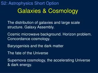
S2: Astrophysics Short Option. Galaxies & Cosmology. The distribution of galaxies and large scale structure. Galaxy Assembly. Cosmic microwave background. Horizon problem. Concordance cosmology. Baryogenisis and the dark matter The fate of the Universe

S2: Astrophysics Short Option
E N D
Presentation Transcript
S2: Astrophysics Short Option Galaxies & Cosmology The distribution of galaxies and large scale structure. Galaxy Assembly. Cosmic microwave background. Horizon problem. Concordance cosmology. Baryogenisis and the dark matter The fate of the Universe Supernova cosmology, the accelerating Universe & dark energy.
The distribution of galaxies The Local Group
Mapping the Universe Hubble’s law: that the distance to a galaxy is proportional to recession velocity provides a way of determining the position of galaxies in 3D. By measuring the 3D positions we can explore how galaxies are distributed in space “the structure of the Universe” Galaxies are not distributed uniformly, but rather found in filaments, on thin sheets and where filaments and sheets meet, in rich clusters. 1995 : CfA Redshift Survey : 15,000 km/s, z=0.05 Thin slice: 6° Thick slice: 36 °
The distribution of galaxies Observations 140Mpc 500Mpc Hot DM Warm DM Cold Dark Matter Cold DM The computer simulations utilising different kinds of dark matter show how the distribution of galaxies tells us about the nature of dark matter. E.g. Neutrinos (HDM) would decouple when they were still relativistic wiping out structure on small scales and producing an expected distribution quite different from that observed. The distribution of galaxies suggests that Cold Dark Matter is required. Warm DM Hot DM
Galaxy Assembly Galaxies were closer together in the past. Strong tidal interactions were more common. Hubble Space Telescope has revealed that find that galaxies with disturbed morphologies are more common in the past. The morphological type is a strong function of local galaxy density with early-type galaxies dominating the galaxy population in the rich clusters. Galaxy interactions play an important role in shaping galaxies.
The Robertson Walker Metric Einstein realised that spacetime would be curved in a Universe filled with matter. If we assume the Universe is homogeneous and isotropic (this is known as the Cosmological Principle) the metric in a curved spacetime is: in spherical polar co-ordinates centred on an observer where r, θ & φ are time independent co-moving co-ordinates and R(t) is the scale factor of the Universe defined so that R=1 today. The k term can take values -1, 0, 1 and is the curvature.
Cosmological time dilation & redshift Define `cosmic proper time’ measured by observers carried along with the expansion. All such clocks must run at the same rate otherwise in some galaxies time would pass faster, stars would have shorter lifetimes and the Universe would not be homogeneous. However when an observer looks at a distant galaxy in an expanding universe the light travel time makes distant clocks appear to run slow. Using the RW metric light signals emitted from galaxy 1 at time intervals Δt1 are received at galaxy 2 at intervals of Δt2 where : Δt2/ Δt1 = R(t2)/R(t1). The Universe was smaller at t1 and so the t2 intervals are longer. Similarly the frequency of waves is reduced and their wavelength increased – the redshift! λ2/ λ1 = c Δt2/ c Δt1 = R(t2)/R(t1) = (1 + z) NB. (i) For nearby galaxies the redshift approximates to a Doppler shift (v/c) but for more distant galaxies. z can be >1. (ii) No light will reach us from further away than the distance light can travel in the age of the Universe. This marks the horizon from which light is infinitely redshifted (R=0). We call this the size of the observable Universe. (iii) Although we cannot see back to the Big Bang the radiation of the cosmic microwave background originates very close to it.
This radiation originates 380,000 years after the Big Bang Cosmic Microwave Background COBE WMAP
Matter & radiation dominated eras The present mass density of the Universe is ~ 2.5 10-27kg/m³ (about 2 protons/m³). At earlier times the mass density was higher by a factor R(t)-3. The present day energy density in CMB photons is 5 105 eV/m³. At earlier times each photon had a higher energy (shorter wavelength) by a factor R(t)-1 and the number density of photons increases by R(t)-3. Thus the energy density of radiation falls faster than the matter energy density. Problem 17 Calculate the energy density in matter today and compare it with the energy Density in the CMB radiation. At what redshift were the two energy densities equal?
Cosmic microwave background Penzias & Wilson working at Bell Labs were not able to eliminate excess noise in their measurements of flux at centimetre wavelengths when they chopped against a cold source. Dicke & Wilkinson at Princeton realised that this was the relic radiation from the Big Bang predicted by Dicke & Gamov in the 1940s. The energy density is about 0.5eVcm-3, about the same as starlight. Penzias & Wilson won the Nobel Prize in 1978 for this discovery. The COBE satellite measured the spectrum of the CMB. It is a perfect black body, T=2.725K: Now the CMB photons have been redshifted and in a Universe 1000 smaller than ours (z=1000) the wavelength would have been 2μ (cf. 2mm) and T=2725K. At this and earlier times there are sufficient ultra-violet photons in the high energy tail of the spectrum to ionise H.
Cosmic microwave background Planck WMAP The free electrons in the ionised plasma at z>1000 scatter photons and make the Universe opaque. What we see is the last scattering surface as the Universe becomes transparent. The current state-of-the-art results on the CMB come from WMAP. In 2009 ESAs Planck mission was launched with better resolution (5 vs 14 arcmin), wider frequency coverage and greater sensitivity than WMAP. Look out for the results!
Cosmic microwave background The re-constructed image from WMAP in galactic co-ordinates (the galactic centre is at the centre of this image) shows the emission from the disk of the Galaxy and a warmer region up to the top right and cooler region to the lower left. These variations are ~ 0.1% (ΔT = 3.365±0.027 mK) and arise from the motion of the solar system with respect to the CMB. The implied velocity of the Local Group with respect to the CMB rest frame is 627±22 km/s. Compare this to the peculiar velocities of galaxies we considered.
Cosmic microwave background What remains once this dipole is removed is the emission from the Galaxy. This can be removed because its spectrum differs from that of the CMB.
Cosmic microwave background What remains once this dipole is removed is the emission from the Galaxy. This can be removed because its spectrum differs from that of the CMB. Once that has been removed the intrinsic fluctuations in the CMB remain. These Are roughly at the level of ± 0.001%. These fluctuations, although very small, are the seeds from which galaxies grow.
The horizon problem The cosmic microwave background is very smooth but this presents us with a problem. Today the limit of the observable universe, our horizon, is: ct0 = 13.7 109 light years. At the time the CMB photons were last scattered, ctCMB = 380,000 years, and the horizon was 380,000 light years. Converting this to present day co-moving co-ordinates the size of the horizon,rH, at z=1000 is given by : rH = ctCMB/R(tCMB) or 3.8 108 light years. Assuming a flat Universe the angular scale on today’s sky corresponds to: Δθ = rH/ct0 = 0.028 radians = 1.6°! At the time of the CMB there could be no causal connection between areas on today’s sky separated by greater angles. So how did the CMB come to be uniform to ~0.001% across the whole sky? This is the first hint that the Universe experienced a rapid expansion phase at very early times: inflation.
Cosmic microwave background We can describe the pattern of fluctuations in the CMB by a superposition of spherical harmonic components and express the result as a power spectrum showing the relative contributions at each angular scale. In order to interpret the CMB we need a physical model to predict the horizon size at the time it was last scattered. Once we have that linear size we can determine the geometry of the Universe (k) because we have a measurement of the angular scale of the fluctuations.
Cosmic microwave background The result is model dependent but if we use the value of H0 from the HST key project we derive the following results: (i) the `total relative density’ is given in units of the critical density (=3H02/8πG) required for a flat Universe ie. k=0. So these results suggest that the Universe is flat. Why is it so? (ii) Only 27% of density is made of matter, only 17% of which (ie. 4% of the total), is baryonic. The rest is non-baryonic dark matter. (iii) The remaining 73% we believe to be dark energy.
The density of baryons Spiral galaxy rotation curves and the analysis of clusters of galaxies suggest that much gravitating mass does not emit EM radiation. This mass cannot be in the form of baryons. At very early times the Universe was dominated by radiation. Massive particles, like baryons, did not exist. As the Universe cooled particles appeared as the energy fell below the rest mass energy of a particular particle. Hence baryons & mesons appeared 10-5s after the Big Bang. In principle more massive nuclei could have been created at this time but there is not enough time when they can be stable. At early times heavy nuclei would be destroyed by high energy photons and later there is insufficient energy to enable fusion. See Liddle `An Intro to Modern Cosmology’ 2nd Ed Ch12
The density of baryons The relative number of protons and neutrons is fixed about 400s after the Big Bang by consideration of the relative masses of n & p and the neutron lifetime (half-life 614s). The ratio Np/Nn = 8. Now the He nucleus is very stable and all the available neutrons are locked into He which has 4mp. If we assume that only H & He are produced we can estimate the mass fraction in He: Y = 2Nn/(Nn + Np) = 2/(1+Np/Nn)= 0.22 The stars and nebulae with very low metal content have Y = 0.23-24. Detailed calculations of the light element abundances in the Big Bang show that the abundance of deuterium is sensitive to the mass density in baryons and indicates a value of 0.04ρc, where ρc = 3H02/8πG, is the critical density. This agrees with the result from the CMB so the dark matter needed to account for 27% matter density is not baryonic.
What is dark matter? • The dark matter is: • non-baryonic • weakly interacting • cold (non-relativistic = not neutrinos) • undetected – but look out LHC results
Newtonian motivation of the Friedman equation Critical density Introduce Λ, the cosmological constant Introduce the fluid equation Show how this can lead to accelerating and decelerating solutions Supernova Cosmology Project Accelerating Universe The horizon problem, the flatness problem & inflation.
Discovering distant supernovae Distant supernovae are discovered by a time sequence of HST images plus co-ordinated spectroscopy to confirm that these are Type1a supernovae (standard candles). These are secondary distance indicators, the intrinsic luminosity is calculated from the apparent brightness and rate of decline.
M = 0 Open M < 1 M = 1 Closed M > 1 fainter - 14 - 9 - 7 today billion years Mean distance between galaxies Time
The Fate of the Universe • When the first high redshift supernovae were discovered in 1998 they were too bright by ~30% to be consistent with a • model with Λ=0 and having all the critical mass in non-baryonic dark matter. • Galaxies were not as close together in the past as the simple decelerating models would predict: the deceleration is slowing. • Accelerating Universe! Confirmed by CMB & galaxy distribution.
Inflation Our best estimate is that: ΩTotal = ΩM + ΩΛ= 1.02 ± 0.02 but ΩM decreases because mass density decreases as the universe expands and ΩΛ (=Λ/3H²) increases with time as the Universe expands. So how is it that these two terms are comparable now? This is known as the flatness problem. • In the early 1980s Alan Guth and others proposed the theory of inflation to account for the horizon problem, the flatness problem and the origin of the CMB fluctuations. • If at early times, t ~ 10-30s, if the value of Λ was very large then the expansion would be dominated by Λ and the Universe would undergo an exponential expansion. • This solves the horizon problem because all parts of the CMB sky would be within the • horizon before inflation and could therefore be causally connected. • Similarly since ΩTotal -1 = ΩM + ΩΛ = kc²/H²R² • And since kc² is constant, & H² = Λ/3 is also constant, then ΩTotal -1 is driven to a very small value by the huge increase in R thus producing a flat universe. • The quantum fluctuations in the pre-inflationary Universe are inflated to become the CMB fluctuations we see today that provide the seed for galaxies.