X-Ray Spectroscopy
X-Ray Spectroscopy. The need for high resolution X-ray spectroscopy Astrophysical Plasmas: Simulation of the emission from a gas at T = 10 7 K with normal abundances of elements. An energy resolution of ~ 10 eV is required to begin serious X-ray spectroscopy and a resolution

X-Ray Spectroscopy
E N D
Presentation Transcript
The need for high resolution • X-ray spectroscopy • Astrophysical Plasmas: • Simulation of the emission from • a gas at T = 107 K with normal • abundances of elements. • An energy resolution of ~ 10 eV • is required to begin serious • X-ray spectroscopy and a resolution • of ~ 1 eV is required for complete • plasma diagnostics and velocity • measurements. 1 eV 10 eV 100 eV Energy (keV)
What’s a milliCrab? • The second brightest X-ray (1-10 keV) source in the sky is the Crab nebula • Its photon intensity at the top of the atmosphere of the Earth is ~ 10 cm-2 s-1 • There are about 1000 AGN (“quasars”) at a level of about .01 cm-2 s-1 =1 mC
Oxygen Shock-Heated to kT ~ 0.3 keV ionized H-like He-like Ionization age
X-Ray Spectrum with 100 eV Resolution 4-6 keV Cassiopeia A ACIS spectrum
X-Ray Spectrometers - I • Proportional counters have • High efficiency • Imaging capability • Multiplex spatial/spectral without confusion But resolving power ≡ E/(δE) ≈ 6√E(keV)
X-Ray Spectrometers - II • Bragg crystal spectrometers • Dispersive, so they can use any detectors • Can achieve R > 103 • Can have high efficiency (at one E at a time) But no imaging or multiplexing capabilities (i.e. can look at only one E at a time)
X-Ray Spectrometers - III • Gratings • Dispersive • Can have moderate (few %) efficiencies • Can multiplex (all E at the same time) • Can have R > 103/√E(keV) (better for low E) But image and spectral orders are mixed
Capella Chandra HETG
X-Ray Spectrometers - IV • Solid State (including CCDs) • High efficiency (>90%) • Non-dispersive, can multiplex all E • Imaging capability without confusion with E But cannot achieve better than R ≈ 25√E(keV) (Resolution ≈ 40√E(keV) eV)
The need for high resolution • X-ray spectroscopy • Astrophysical Plasmas: • Simulation of the emission from • a gas at T = 107 K with normal • abundances of elements. • An energy resolution of ~ 10 eV • is required to begin serious • X-ray spectroscopy and a resolution • of ~ 1 eV is required for complete • plasma diagnostics and velocity • measurements. 1 eV 10 eV 100 eV Energy (keV)
X-Ray Spectrometers - V • Cryogenic Microcalorimeters • High efficiency (>90%) • Non-dispersive, can multiplex all E • Imaging capability without confusion with E And can achieve R > 103 √E(keV)
w Expected with XRS (12 eV) He-like Fe He-like Fe “triplet” y, x z Neutral Fe w x H-like Fe Counts z y Chandra HEG (~ 60 eV) Energy (keV) Physical Conditions Through X-Ray Spectroscopy Fe-K lines provide very clean diagnostics. One such diagnostic: excellent density-independent temperature sensitivity in the range 107–108 Kelvin.
The X-ray Microcalorimeter Features high resolution, non-dispersive spectroscopy with high quantum efficiency over K- and L- atomic transition band. Moseley, Mather and McCammon 1984
Simple Energy Resolution Argument • δT = E/C (temperature rise for E deposition) • C ≈ N(kT)/T (N = # of phonons with <kT>) • N ≈ C/k (fluctuation in N is the “noise”) • ΔN = √N (Poisson statistics) • R = E/(ΔE) (resolving power) • ΔE ≈ kT√N ≈ kT√(C/k) ≈ √(kT2C) • More carefully, ΔE = 2.35 ζ √(kT2C)
Spectral Resolving Power: Depends on thermometer technology Temperature-sensitive resistance Resolution limited by thermal fluctuations between sensor and heat bath and Johnson noise. Doped semiconductor R (ohms) Temperature T = operating temperature (50-100 mK) C = heat capacity • ~ 2 - 4 for doped semiconductors ~ 0.2for transition edge sensors For both thermometer schemes a spectral resolution of few a eV is possible! R (ohms) Superconducting Transition Temperature
Basic requirements: • • Low temperature • • Sensitive thermometer • • Thermal link weak enough that the time for restoration of the base temperature is the slowest time constant in the system yet not so weak that the device is made too slow to handle the incident flux. • • Absorber with high cross section yet low heat capacity • • Reproducible and efficient thermalization Types of thermometers: • resistive • capacitive • inductive • paramagnetic • electron tunneling
. . . Microcalorimeter Arrays XQC Array: 36 array of 0.5 2 mm pixels.
E 6.4 eV FWHM Ion beam 1.5 m Energy (keV) (after anneal) ~ 6 times deeper thermometer Deep implants using silicon-on-insulator wafers. 625 m pixels GSFC Mn Ka1 Mn Ka2
RTS – Rotating Target Source X-ray lines continuum X-ray source X-ray continuum rotating target wheel targets (one is open for continuum)
motor target wheel