Predicate Logic
Predicate Logic. From Propositional Logic to Predicate Logic. Last week, we dealt with propositional (or truth-functional) logic: the logic of truth-functional statements. Today, we are going to deal with predicate (or quantificational) logic.

Predicate Logic
E N D
Presentation Transcript
From Propositional Logic to Predicate Logic • Last week, we dealt with propositional (or truth-functional) logic: the logic of truth-functional statements. • Today, we are going to deal with predicate (or quantificational) logic. • Quantificational logic is an extension of, and thus builds on truth-functional logic.
Recap: Formal Logic • Step 1: Use certain symbols to express the abstract form of certain statements • Step 2: Use a certain procedure based on these abstract symbolizations to figure out certain logical properties of the original statements.
Recap: Truth Tables • Truth-Tables • Slow • Systematic • Reveals consequence as well as non-consequence • Only works for truth-functional logic
Recap: Formal Proofs • Formal Proofs • Pretty fast (with practice!) • Not systematic • Can only reveal consequence • Can be made into systematic method (that can then also check for non-consequence) but becomes inefficient • Can be used for predicate logic
Recap: Truth Trees • Truth Trees • Fast • Systematic • Can reveal consequence as well as non-consequence • Can be used for truth-functional as well as predicate logic
Individual Constants • An individual constant is a name for an object. • Examples: john, marie, a, b • Each name is assumed to refer to a unique individual, i.e. we will not have two objects with the same name. • However, each individual object may have more than one name.
Predicates • Predicates are used to express properties of objects or relations between objects. • Examples: Tall, Cube, LeftOf, = • Arity: the number of arguments of a predicate (E.g. Tall: 1, LeftOf: 2)
Interpreted and Uninterpreted Predicates • Just as ‘P’ can be used to denote any statement in propositional logic, a predicate like ‘LeftOf’ is left ‘uninterpreted’ in predicate logic. Thus, a statement like LeftOf(a,a) can be true in predicate logic. • The predicate ‘=‘ is an exception: it will automatically be interpreted as the identity predicate.
Quantification: ‘All’ and ‘Some’ • In quantificational logic, there are two quantifiers: ‘all’ and ‘some’. • Here are some examples: • x Mortal(x) ‘All things are mortal’ • x Mortal(x) ‘Some things are mortal’ • x (Human(x) Mortal(x)) ‘Every human is mortal’ • x (Human(x) Mortal(x)) ‘Some human is not mortal’
The Four Aristotelian Forms • “All P’s are Q’s” • x (P(x) Q(x)) • “Some P’s are Q’s” • x (P(x) Q(x)) • “No P’s are Q’s” • x (P(x) Q(x)) • “Some P’s are not Q’s” • x (P(x) Q(x))
Swapping Mixed Quantifiers: Order Matters y x Likes(x,y) “Something is liked by everything (including itself)” x y Likes(x,y) “Everything likes something (possibly itself)”
Expressing Number of Objects • How do we express that there are (at least) two cubes? • Note that x y (Cube(x) Cube(y)) doesn’t work: this will be true in a world with 1 object (just pick that object for both x and y!) • So, we have to make sure that x and y are different objects: x y (xy Cube(x) Cube(y))
‘Exactly One’ • How can we say that “There is exactly one cube”? • Saying that there is exactly one cube is saying two things at once: • There is at least one cube: xCube(x) • There is at most one cube: xy(Cube(x)Cube(y) xy) • Thus: xCube(x) xy(Cube(x)Cube(y)xy) • Alternatively (and simpler): • x(Cube(x) y(Cube(y) xy)) • x(Cube(x) y(Cube(y) x=y)) • x y(Cube(y) x=y))
‘Exactly Two’ • How do we say “There are exactly two cubes”? • Similar set-up: • x y(Cube(x) Cube(y) xy z(Cube(z) zx zy)) or: • x y(Cube(x) Cube(y) xy z(Cube(z) (z=x z=y))) or: • x y(xy z(Cube(z) (z=x z=y)))
Quantifier Negation Equivalences • x P(x) x P(x) • x P(x) x P(x) • Sometimes these are called the DeMorgan Rules for Quantifiers, which makes sense: • x P(x) P(a) P(b) … • x P(x) P(a) P(b) …
Rewriting Example If x (P(x) Q(x)) (‘not all P’s are Q’s), then x (P(x) Q(x)) (some P’s are not Q’s), and vice versa: x (P(x) Q(x)) (QN) x (P(x) Q(x)) (Impl) x (P(x) Q(x))
Other Quantifier Equivalences • over , and over : • x ((x) (x)) x (x) x (x) • x ((x) (x)) x (x) x (x) • Null Quantification: • x P P • x P P • Replacing bound variables: • x (x) y (y) • x (x) y (y) • Swapping quantifiers of same type: • x y (x,y) y x (x,y) • x y (x,y) y x (x,y)
The Assumption of Existential Import • The Assumption of Existential Import is the assumption that the world in which we evaluate is not empty, i.e. that at least one thing exists. • Under this assumption, x P(x) is true if x P(x) is true. Without the assumption, however, it’s not: if the world in which we evaluate is empty, then x P(x) is false, even though x P(x) is (vacuously) true. • In first-order logic, we usually make the assumption of existential import. Thus, x P(x) is considered a FO consequence of x P(x), even though logically it is not.
Quantifier Rules in F • There are 4 quantifier rules in F: • Universal Introduction and Elimination • Existential Introduction and Elimination • Universal Introduction and Existential Elimination have important restrictions in that the rules cannot be applied relative to just any individual constant. The system F deals with those restrictions through the use of subproofs. We’ll see later how that works. • Fortunately, Universal Elimination and Existential Introduction do not have any restrictions, so we’ll start with those.
Notation • In describing the rules, the following notation is useful: • (x) is a wff with zero or more instances of x as the only free variable. • (a/x) is the statement that results when substituting ‘a’ for all occurrences of ‘x’ that are free in (x). • If it is clear which variable we are subsituting, we will simply write (a).
Elim • Universal Elimination ( Elim) allows one to conclude that any thing has a certain property if everything has that property: x (x) (a)
Good and Bad Uses of Elim x SameSize(x,x) x SameSize(x,x) Good Bad SameSize(a,a) SameSize(a,b) • The same individual constant should be used! x SameSize(x,x) x (Tet(x) x Large(x)) Bad Bad SameSize(x,a) Tet(a) x Large(a) • Only free occurrences of x should be replaced! • All free occurrences of x should be replaced!
Intro • Existential Introduction ( Intro) allows one to conclude that something has a certain property if some thing has that property: (a) x (x)
Good and Bad Uses of Intro SameSize(a,a) SameSize(a,a) Good Good x SameSize(x,x) x SameSize(a,x) • Not all occurrences of a have to be replaced! SameSize(a,b) x SameSize(a,x) Bad Bad x SameSize(x,x) x x SameSize(x,x) • Doesn’t follow the rule (no free x’s in x SameSize(x,x)) • The same individual constant should be used!
Universal Proof • A common proof in mathematics is a universal proof. • A universal proof proves something about everything (of the Universe of Discourse) by proving it to be true of some arbitrary thing. • It usually starts with “Let ‘a’ be an arbitrary …” • It then proves something about ‘a’ • Finally, since ‘a’ was just an arbitrary individual, it must be true for all individuals.
Intro • Universal Introduction ( Elim) allows one to conclude that everything has a certain property if anything has that property: a a may not occur before the subproof, unless all subproofs in which it occurs have been closed. a may not occur in (x) either. (a) x (x)
Good and Bad Uses of Intro Tet(a) a a Good Bad SameSize(a,a) SameSize(a,a) x SameSize(x,x) x SameSize(x,x) • a occurs before subproof! a Still Good a Tet(a) Bad SameSize(a,a) x Tet(x) x SameSize(a,x) • a occurs outside subproof, but only in a subproof that has been closed. • a occurs in SameSize(a,x)!
Existential Proof • Sometimes, we know that something has a certain property, but we don’t know who or what this something is. • In order to perform some reasoning, we will give this something a name, and whatever we can infer from that point on, we can infer from the original statement. • Like the universal proof, the name should be an arbitrary name, but in this case it denotes a specific individual: that individual that had the relevant property.
Elim • Existential Elimination ( Elim) allows one to conclude anything that follows from some thing having a certain property, given that something has that property. x (x) a (a) a may not occur before the subproof, unless all subproofs in which it occurs have been closed. a may not occur in Q either. Q Q
Good and Bad Uses of Elim x SameSize(x,x) Tet(a) a SameSize(a,a) x SameSize(x,x) Good Bad a SameSize(a,a) x Cube(x) x Cube(x) x Large(x) a Cube(a) x Large(x) Still Good • a occurs before subproof! Tet(b) a SameSize(a,a) Tet(b) Bad • a occurs before subproof, but only in a subproof which has been closed. Large(a) Large(a) • a occurs in Large(a)!
= Intro • At any point, you can assert any statement of the form a=a • = Intro does not require any statements as part of its justification, and reflects the reflexivity of identity. a = a = Intro
= Elim • = Elim: If you have a statement of the form a=b, and a statement in which a occurs (written as P(a)), then you may infer P(b), which is the statement that results when replacing any number of occurences of a by b in the statement P(a): n P(a) m a = b P(b) = Elim n,m
Rules for other Predicates • Of course, one could define inference rules for predicates other than ‘=‘. For example, given the reflexivity of the SameSize relationship, one could make it a rule that SameSize(a,a) can be inferred at any time. • However, ‘=‘ is the only predicate for which F has defined inference rules as it is the only interpreted predicate. • We’ll see later how we can deal with logical truths about other predicates.
Running Examples Valid Argument x (Cube(x) Small(x)) x Cube(x) x Small(x) Invalid Argument x Cube(x) x Small(x) x (Cube(x) Small(x))
Truth-Functional Expansions • Suppose that our Universe of Discourse (UD) contains only the objects a and b. • Given this UD, the claim x Cube(x) is true iff Cube(a) Cube(b) is true. • Similarly, the claim x Cube(x) is true iff Cube(a) Cube(b) is true. • The truth-functional interpretation of the FO statements given a fixed UD is called the truth-functional expansion of the original FO statement with regard to that UD.
Truth-Functional Expansions and Proving FO Invalidity • Truth-Functional expansions can be used to prove FO invalidity. Example: x Cube(x) x Small(x) x (Cube(x) Small(x)) UD = {a,b} T T F T F T T (Cube(a) Cube(b)) (Small(a) Small(b)) (Cube(a) Small(a)) (Cube(b) Small(b)) T F F F F F T This shows that there is a world in which the premise is true and the conclusion false. Hence, the original argument is FO invalid.
Truth-Functional Expansions and Proving FO Validity • If the truth-functional expansion of an FO argument in some UD is truth-functionally invalid, then the original argument is FO invalid, but if it is truth-functionally valid, then that does not mean that the original argument is FO valid. • For example, with UD = {a}, the expansion of the argument would be truth-functionally valid. In general, it is always possible that adding one more object to the UD makes the expansion invalid. • Thus, we can’t prove validity using the expansion method, as we would have to show the expansion to be valid in every possible UD, and there are infinitely many UD’s. • The expansion method is therefore only good for proving invalidity. Indeed, it searches for countermodels.
The Expansion Method as a Systematic Procedure • Still, what is nice about the expansion method is that it can be made into a systematic procedure: • Step 1: Expand FO argument (which can be done systematically) in UD = {a}. • Step 2: Use some systematic procedure (e.g. truth-table method or truth-tree method) to test whether the expansion is TF invalid. If it is TF invalid, then stop: the FO argument is FO invalid. Otherwise, expand FO argument in UD = {a,b}, and repeat step 2.
Incompleteness of the Expansion Method • We saw that the expansion method is not a test for FO validity, but only for invalidity. • However, even as such it is an incomplete test! • Proof: Consider the following argument: xy(xy ((x>y y>x) (x>y y>x))) xyz((x>y y>z) x>z) xy(xy x>y) For any UD with an arbitrarily large yet finite number of objects, the expansion of this argument will be truth-functionally valid. However, the argument is FO invalid (consider the natural numbers)!
A More Focused Search • A further drawback of the expansion method is that the search for a counterexample is very inefficient. • A focused search for a counterexample is more efficient: • (for the invalid argument) I want there to be at least one cube, and at least one small object, but no small cubes. So, if we have a cube, a, then a cannot be small, so I need a second object, b, which is small, but not a cube. Counterexample, so the argument is invalid.
Advantage of a Focused Search • The focused search method is like the indirect truth-table method. • Indeed, like the indirect truth-table method, the focused search method can prove validity: • (for the valid argument) I want there to be at least one small cube. Let us call this small cube a. How, I don’t want it to be true that there is at least one cube and at least one small object. However, a is both a cube and small. Contradiction, so I can’t generate a counterexample.
Truth-Trees for Predicate Logic • Like the direct method, the focused search method needs to be systematized, especially since the search often involves making choices. • Fortunately, the truth-tree method, which systematized the indirect truth-table method in truth-functional logic, can be extended for predicate logic.
Truth-Tree Rules for Quantifiers x (x) x (x) x (x) x (x) x (x) x (x) (c) (c) with ‘c’ any constant with ‘c’ a new constant in that branch
Truth-Tree Rules for Identity (c) a a c = d (or d = c) × (d) (where (d) is the result of replacing any number of c’s with d’s in (c))
Truth-Tree Example I x Cube(x) x Small(x) x (Cube(x) Small(x)) x Cube(x) x Small(x) x (Cube(x) Small(x)) Cube(a) Small(b) (Cube(a) Small(a)) (Cube(b) Small(b)) Cube(a) Small(a) × Cube(b) Small(b) Open branch, so it’s invalid ×