Today in Astronomy 102: relativity and the Universe

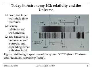
1. Today in Astronomy 102: relativity and the Universe • From last time:wormhole time machines • General relativity and the Universe. • The Universe ishomogeneous, isotropic, and expanding; what is its structure? • Figure: visible-light spectrum of the quasar 3C 273 (from Chaisson and McMillan, Astronomy Today). Astronomy 102, Fall 2001

2. How to build a wormhole time machine • Start with a wormhole whose two mouths (called mouths A and B) are close together in space. Fix things up so that they stay the same distance apart in hyperspace. • In Thorne’s description in the book, this is illustrated by two people reaching into each mouth to hold hands. • Take mouth B on a trip at high speeds (approaching light speed), out a great distance, and then back to its former spot, without ever changing the distance between the two mouths in hyperspace. Astronomy 102, Fall 2001

3. How to build a wormhole time machine (continued) Mouth B Mouth A B takes a trip at relativistic speeds …and returns to its original position Astronomy 102, Fall 2001

4. How to build a wormhole time machine (continued) • Because of time dilation, the trip will take a short time according to an observer travelling with mouth B, and a much longer time according to an observer who stays with the “stationary” mouth A. • While B is gone, the observer at A can travel into the future (to the time when B returns) by passing through mouth A. • After B returns, an observer at B can travel into the past (to the time when B left) by passing through mouth B. • The length of time travel is thus the time lag between clocks fixed to A and B during B’s trip, and is thus adjustable by adjusting the details of the trip. • Travel between arbitrary times is not provided! Astronomy 102, Fall 2001

5. Odd features of time travel • Paradoxes such as the “matricide paradox” come up! One could use a time machine, for example, for travelling back through time before one’s birthday and killing one’s mother. • Does physics prevent one from being born and travelling back through time in the first place? • Maybe. How is it that one can start with laws of physics like the Einstein field equation, that have cause and effect built in, and derive from them violations of cause and effect? • Maybe not. What about quantum mechanics? Vacuum fluctuations, for instance, have no “cause.” If quantum behavior (associated with singularities) is inherent in the wormhole, one could still exist after committing paradoxical matricide. Astronomy 102, Fall 2001

6. Alas, it may be impossible to build a stable wormhole time machine • Geroch, Wald, and Hawking on self-destruction of wormhole time machines: • Light leaving the origin during B’s trip, and entering mouth B as it is returning, can travel backwards in time, emerge from A, and meet itself in the act of leaving. • It can do this as many times as it likes, even an infinite number of times. • Since light can interfere constructively (all the peaks and troughs of the light wave lining up), a large positive energy density could be generated in the wormhole, which would collapse it. • This process could take as little as 10-95 seconds in the frame of reference of mouth A. Astronomy 102, Fall 2001

7. A recipe for wormhole time-machine destruction A (past) B (future) Light emerging from mouth A Aim a laser at mouth B; orient mirror so that light emerging from mouth A joins up with the beam aimed at mouth B. Laser Immediately a huge number of photons emerges from mouth A, and the vast increase of energy inside it collapses the wormhole. Mirror Astronomy 102, Fall 2001

8. Alas, it may be impossible to build a stable wormhole time machine (continued) • It’s also possible for this to happen with light created by vacuum fluctuations!. • Since light has wave properties too, the probability that virtual photons from near A to travel to B and re-emerge from A pointed again at B is not zero, even if there is nothing to aim the photons that way. • The interference may not be constructive, though, because the wormhole tends to defocus the light in the manner of a negative lens; therefore we do not know whether this is a fatal objection. Astronomy 102, Fall 2001

9. Mid-lecture Break. • Remember, homework #6 is due tomorrow, Friday, 30 November 2001, at 11 PM. • Here’s what you missed by not gettingup before 5AM on Sunday, 11/18, to seethe Leonid meteorshower. (From APOD;photo by Jerry Lodriguss.) Astronomy 102, Fall 2001

10. General relativity and the Universe • It was recognized soon after Einstein’s invention of the general theory of relativity in 1915 that this theory provides the best framework in which to study the large-scale structure of the Universe: • Gravity is the only force known (then or now) that is long-ranged enough to influence objects scales much larger than typical interstellar distances. All the other forces (electricity, magnetism and the nuclear forces) are “shielded” in large accumulations of material or are naturally short ranged. • And there’s lots of matter around to serve as gravity’s source. • Einstein himself worked on this application of GR, rather than on “stellar” applications like black holes. The results wind up having a lot in common with black holes, though. Astronomy 102, Fall 2001

11. The Universe contains: PlanetsEarth’s diameter = 1.3104 km StarsSun’s diameter = 1.4106 km Planetary systemsSolar system diameter = 1.21010 km Star clusters, interstellar cloudsTypical distance between stars = a few light years (ly) = 31013 km GalaxiesDiameter of typical galaxy = a hundred thousand ly = 1018 kmTypical distance between galaxies = a million light years (Mly) = 1019 km It was long thought by most scientists that the nebulae we now call galaxies were simply parts of the Milky Way. In the early 1920s Edwin Hubble measured their distances and proved otherwise. Basic structure of the Universe Astronomy 102, Fall 2001

12. The Universe is full of galaxies, and to observethem is to probe the structure ofthe Universe. • This is part of the northern HST Deep Field (NASA/STScI). • Only a few stars are present; virtually every dot is a galaxy. If the whole sky were imaged with the same sensitivity and the galaxies counted, we’d get about 100 billion. Astronomy 102, Fall 2001

13. General relativity and the structure of the Universe • The Universe is not an isolated, distinct object like those we’ve dealt with hitherto. In its description we would be interested in the large-scale patterns and trends in gravity (or spacetime curvature). Why? • These trends would tell us how galaxies and groups of galaxies – the most distant and massive things we can see – would tend to move around in the Universe, and why we see groups the size we do: this study is called cosmology. • They might also tell us about the Universe’s origins and fate: this is called cosmogony. • By large-scale, we mean sizes and distance large compared to the typical distance between galaxies. Astronomy 102, Fall 2001

14. General relativity and the structure of the Universe (continued) • To solve the Einstein field equation for the Universe one needs to apply what is known observationally about the Universe, as “initial conditions” or “boundary conditions.” The solutions will tell us the conditions for other spacetime points or conditions. • And in the early 1920s observations (by Edwin Hubble, again) began to suggest that the distribution of galaxies, at least in the local Universe, is isotropic and homogeneous on large scales. • Isotropic = looks the same in all directions from our viewpoint. • Homogeneous = looks the same from any viewpoint within the Universe. • These facts serve as useful “boundary conditions” for the field equation. Astronomy 102, Fall 2001

15. Isotropy of the Universe on large scales: modern measurements Here positions are marked for galaxies lying within a 6ox6o patch of the sky: the galaxies are essentially randomly, and uniformly, distributed. (From F. Shu, The Physical Universe.) For scale: 0.5o (size of the full moon) Astronomy 102, Fall 2001

16. Isotropy of the Universe on large scales: modern measurements (continued) • Isotropy on the scale represented by these circles’s diameter means that approximately the same numbers of galaxies are contained within them, no matter where on the sky we put them, which is evidently true in this picture. Astronomy 102, Fall 2001

17. Homogeneity of the Universe on large scales: modern measurements • The Las Campanas Redshift Survey, showing the positions, out to distances of about 3x109 light years along the line of sight, of almost 24,000 galaxies in six different thin stripes on the sky. Data from stripes in the northern and southern sky are overlaid. Again, the galaxies and their larger groupings tend to be randomly distributed through volume on large scales. From Huan Lin, U. Toronto. Astronomy 102, Fall 2001

18. Homogeneity of the Universe on large scales: modern measurements (continued) • Homogeneity on the scale of these circles’s diameter means that approximately the same numbers of galaxies are contained within them, no matter where we put them within the Universe’s volume, which is evidently true in this picture. • Hubble actually did it a bit differently: he observed that fainter galaxies (same as brighter ones, but further away) appear in greater numbers than brighter galaxies, by the amount that would be expected if the galaxies are distributed uniformly in space. Astronomy 102, Fall 2001

19. Back to general relativity and the structure of the Universe … • Einstein and de Sitter (late 1910s and 1920s, Germany), Friedmann (1922, USSR), Lemaitre (1927, Belgium), and Robertson and Walker (1935, US/UK) produced the first solutions of the field equations for an isotropic and homogeneous Universe. • The types of solutions they found: • Collapse, ending in a singularity. • Expansion from a singularity, gradually slowing and reversing under the influence of gravity, ending in a collapse to a singularity.This, and the previous outcome, are for universes with total kinetic energy (energy stored in the motions of galaxies) less than the gravitational binding energy. They are called closed universes. Astronomy 102, Fall 2001

20. General relativity and the structure of the Universe (continued) • Expansion from a singularity, that gradually slows, then stops. (Total kinetic energy = gravitational binding energy.)This is generally called a marginal, or critical, Universe. • Expansion from a singularity, that continues forever (total kinetic energy greater than gravitational binding energy). This is called an open universe. Model 1 is of course a lot like what we now call black hole formation, since it ends in a singularity. Note that models 2-4 all involve expansion from asingularity, so the creation and development of the Universe must be rather like black hole formation running in reverse. Astronomy 102, Fall 2001

21. Einstein doesn’t like it. • All the solutions have these features in common: • singularities, and • dynamic behavior: the structure given by the solutions is different at different times between singularities (at which time doesn’t exist, of course). • Einstein thought that singularities such as these indicated that there were important physical effects not accounted for in the field equation. He also thought that the right answer would involve static behavior: large-scale structure should not change with time. • He also saw how he could “fix” the field equation to eliminate singular and dynamic solutions: introduce an additional constant term, which became known as the cosmological constant, to represent the missing, unknown, physical effects. Astronomy 102, Fall 2001

22. The field equation and the cosmological constant: hieroglyphics (i.e. not on the exam or homework) • The field equation under a particularly simple set of assumptions and conditions for a homogeneous and isotropic Universe: • The same equation modified by Einstein (1917): Spacetimecurvature Typical distance between galaxies Mass per unit volume Cosmological constant A certain positive value of  leadsa static solution. Astronomy 102, Fall 2001

23. Edwin Hubble strikes again: the Universe expands. • Then, in 1929, Hubble made his third great contribution to cosmology; he observed that: • distant galaxies are always seen to have redshifted spectra. Thus they all recede from us. • the magnitude of this Doppler shift for any given distant galaxy is in direct proportion to the distance to this galaxy: with V = velocity and D = distance to galaxy,where H0 = 20 km/sec/Mly according to the most recent measurements by the Hubble Space Telescope. • This means that the Universe is expanding. (Hubble’s Law) Astronomy 102, Fall 2001

24. Relation between galaxy redshift and distance • Visible-light spectra (left) of several different galaxies (right). The extent of the redshift, denoted by the horizontal yellow arrows, and the distance to each galaxy (in the center) increase from top to bottom. 1 parsec = 3.26 ly. • (Figure: Chaisson and McMillan, Astronomy Today.) Astronomy 102, Fall 2001

25. Einstein gives up. • The Universe is observed to be expanding; it is not static. • Thus the real Universe may be described by one of the dynamic solutions to the original Einstein field equation. Of the four types we discussed above, the last three spend at least part of their time, if not all, expanding. • Thus there appeared to be no point in Einstein’s cosmological constant, so he let it drop, calling it “my greatest blunder.” • Thereafter he began trying to show that the singularities in the dynamic solutions simply wouldn’t be realized. His effort resulted in the steady-state model of the Universe, which we’ll describe later. • This isn’t the last we’ll see of the cosmological constant, though. Astronomy 102, Fall 2001

26. Possibilities for the structure of the expanding Universe Unbound (open) Typical distance between galaxies Marginal (total kinetic energy = binding energy) Bound (closed) Big Bang Big Squeeze Time All three expanding solutions predict that the matter in the universe was concentrated at earlier times, and that the expan-sion started as an explosion of this concentration: the Big Bang. Astronomy 102, Fall 2001

27. Possibilities for the structure of the expanding Universe (continued) Unbound (open) Typical distance between galaxies Marginal (total kinetic energy = binding energy) Bound (closed) Time To tell which solution describes the real Universe, we need to measure the acceleration of the galaxies as well as their velocities. Astronomers have been working on this for decades. Astronomy 102, Fall 2001