Download

1 / 249
2.54k likes | 2.89k Vues
MICROECONOMICS Classroom Lecture Notes (3 credits, as of 2005). based on Hal R. Varian’s Intermediate Microeconomics , Sixth Edition, referring to Pindyck and Rubinfeld’s Microeconomics , Fourth Edition. Chapter 0 . Economics. The source of all economic problems is scarcity.

E N D
MICROECONOMICSClassroom Lecture Notes (3 credits, as of 2005)
based on Hal R. Varian’s Intermediate Microeconomics, Sixth Edition, referring to Pindyck and Rubinfeld’s Microeconomics, Fourth Edition.
Chapter 0 Economics
Problem of trade-off, and choice. Economics, as a way of thinking, as a dismal science. Problems - solutions - hidden consequences.
Main decision-making agents: 1 individuals(household), 2 firms, and 3 governments.
Objects of economic choice are commodities, including goods and services.
Main economic activities: Consumption, Production, and Exchange.
Microeconomics and macroeconomics: to show the market mechanism (the invisible hand), to supplement it.
The circular flow of economic activities. product market factor market
The product market and the factor market. The market relation is mutual and voluntary. Positive issuesand normative issues.
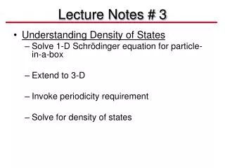
Marginal analysis • Relationsbetween • Total magnitudes, • Average magnitudes, and • Marginal magnitudes.
1, MM is the slope of the TM curve; 2, AM is the slope of the ray from the origin to the point at the TM curve; TM MM(x*) AM(x*) x x*
3, TM increasing (decreasing) if and only if MM > 0 ( MM < 0 ); 4, If TM is at maximum or minimum, then MM = 0;
5, AM increasing (decreasing) if and only if MM > AM ( MM < AM ); 6, If AM is at maximum or minimum, then MM = AM, or MM cuts AM at the latter’s maximum or minimum.
Chapter 1 The Market
Economics proceeds by developing Models of social phenomena. By a model we mean a simplified representation of reality.
Exogenous variables: taken as determined by factors not discussed in a model. Endogenous variables: determined by forces described in the model.
The optimization principle: People try to choose what’s best for them. The equilibrium principle: Prices adjust until demand and supply are equal.
The demand curve: A curve that relates the quantity demanded to price. The reservation price: One’s maximum willingness to pay for something.
From people's reservation prices to the demand curve. Fig. Similarly, the supply curve.
Pareto efficiency: A Pareto improvement is a change to make some people better off without hurting anybody else. A concept to evaluate different ways of allocating resources.
An economic situation is • Pareto efficient • or • Pareto optimal • if there is already no way to make any more Pareto improvement.
Short run and long run • Equilibria in the short run (some factors are unchanged) and in the long run.
Chapter 2 Budget Constraint
* Vector variables and vector functions. • * The inner product of two vectors. • * With theprice vector p = ( p1, …, pn ), the value of the commodity bundle x = ( x1, …, xn ) is pTx = Σi pixi. However, two goods are often enough to discuss.
The budget constraint: p1 x1 + p2 x2 ≤ m. • The budget line and the budget set (the market opportunity set).
The slope of the budget line: d x2 /d x1 = – p1 / p2 . • How the budget line moves when the income changes, or when a price changes.
Budget line andbudget set x2 m/p2 Budget line Slope = -p1/p2 Budget set m/p1 x1
Increasing income x2 m’/p2 Budget line m/p2 Slope = - p1/p2 x1 m/p1 m’/p1
Increasing price m/p2 Budget line Slope = - p1/p2 Slope = - p’1/p2 m/p’1 m/p1
Taxes,quantity taxes, value taxes (ad valorem taxes), and lump-sum taxes. A subsidy is the opposite of a quantity tax. Rationing. Their effects on the budget set.
Chapter 3 Preferences
* Prerequisite: A binary relation R on X is said to be Complete if xRy or yRx for any pair of x and y in X; Reflexive if xRx for any x in X; Transitive if xRy and yRz imply xRz.
Rational agents and stable preferences • Bundle x is strictly preferred (s.p.), or weakly preferred (w.p.), or indifferent (ind.), to Bundle y. (If x is w.p. to y and y is w.p. to x, we say x is indifferent to y.)
Assumptions about Preferences Completeness: x is w.p. to y or y is w.p. to x for any pair of x and y. Reflexivity: x is w.p. to x for any bundle x. Transitivity:If x is w.p. to y and y is w.p. to z, then x is w.p. to z.
The indifference sets, the indifference curves. Fig. They cannot cross each other.
indifference curves x2 x1
Perfect substitutes and perfect complements. Goods, bads, and neutrals. Satiation. • Figs
Perfect substitutes Blue pencils Indifference curves Red pencils
Perfect complements Left shoes Indifference curves Right shoes
Well-behaved preferences are monotonic (meaning more is better) and • convex (meaning average are preferred to extremes). • Figs
Monotonicity x2 Better bundles Better bundles (x1, x2) x1
The marginal rate of substitution (MRS) measures the slope of the indifference curve. • MRS = d x2 / d x1, the marginal willingness to pay ( how much to give up of x2 to acquire one more of x1 ). • Usually negative. • Fig
Convex indifference curves exhibit a diminishing marginal rate of substitution. • Fig.
Convexity x2 (y1,y2) Averaged bundle (x1,x2) x1
Chapter 4 Utility (as a way to describe preferences)
Utilities • Essential ordinal utilities, versus • convenient cardinal utility functions.
Cardinal utility functions: u ( x ) ≥ u ( y ) if and only if bundle x is w.p. to bundle y. • The indifference curves are the projections of contours of u = u ( x1, x2 ). Fig.