Download
1 / 42
420 likes | 535 Vues
Cosmological Constraints from the SDSS maxBCG Cluster Sample. Eduardo Rozo. UC Berkeley, Feb 24, 2009. People: Erin Sheldon David Johnston Risa Wechsler Eli Rykoff Gus Evrard Tim McKay Ben Koester Jim Annis Matthew Becker Jiangang-Hao Joshua Frieman Hao-Yi Wu. . Summary.

E N D
Cosmological Constraints from the SDSS maxBCG Cluster Sample Eduardo Rozo UC Berkeley, Feb 24, 2009
People: Erin Sheldon David Johnston Risa Wechsler Eli Rykoff Gus Evrard Tim McKay Ben Koester Jim Annis Matthew Becker Jiangang-Hao Joshua Frieman Hao-Yi Wu.
Summary • maxBCG contraints are tight: 8(M/0.25)0.41= 0.8320.033. • maxBCG constraints are comparable to and consistent with those derived from X-ray studies. • maxBCG constraints are consistent with WMAP5. Joint constraints are: 8 = 0.8070.020, M = 0.2650.016. • Cluster abundances can help constrain the growth of structure. As such, they are an important probe of modified gravity scenarios. • Follow up observations can help, but we must be smart about it.
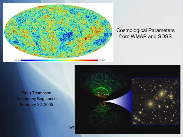
The Broad Brush Background Our protagonist is 8, a measure of how clumpy the matter distribution of the universe is. High 8 - Universe is very clumpy. Low 8 - Universe is more homogeneous. Why is this measurement important? - It can help constrain dark energy. CMB measures inhomogeneities at z~1200. Given the CMB, general relativity, and a dark energy model, we can predict how inhomogeneous the local universe is. By comparing CMB prediction to local measurements of 8 we can constrain dark energy models.
How to Measure 8 with Clusters The number of clusters at low redshift depends sensitively on 8. 8=1.1 Number Density (Mpc-3) 8=0.9 8=0.7 Mass
Why is Measuring 8 Difficult? The main difficulty is that mass is not directly observable. One measures cluster abundances as a function of a mass tracer . We must understand how relates to cluster mass. Two approaches: Understand P(|M) as best as possible a-priori (e.g. Mantz et al. 2008, Henry et al. 2008, Vikhlinin et al. 2008). Parameterize P(|M), and simultaneously fit for these parameters in addition to cosmology. We must supplement cluster abundance data with other mass-sensitive observables, e.g. M|, ln M|, b(), etc.
maxBCG maxBCG is a red sequence cluster finder - looks for groups of uniformly red galaxies.
The maxBCG Catalog maxBCG is a red sequence cluster finder - looks for groups of uniformly red galaxies. • Catalog covers ~8,000 deg2 of SDSS imaging with 0.1 < z < 0.3. • Richness N200 = number of red galaxies brighter than 0.4L* (mass tracer). • ~13,000 clusters with ≥ 10 (roughly M200c~3•1013 M). • 90% pure. • 90% complete. Main observable: n(N200)- no. of clusters as a function of N200.
Other Data - The maxBCG Arsenal • Lensing: measures the mean mass of clusters as a function of richness (Sheldon, Johnston). • X-ray: measurements of the mean X-ray luminosity of maxBCG clusters as a function of richness (Rykoff, Evrard). • Velocity dispersions: measurements of the mean velocity dispersion of galaxies as a function of richness (Becker, McKay).
Collecting the Data: Cluster Stacking Lensing, X-ray, and velocity dispersion data are all based on cluster stacking: Select all clusters of a given richness. Stack all fields (SDSS/ROSAT) to measure the mean weak lensing/X-ray signal of the clusters. Repeat procedure along random points, and subtract uncorrelated background.
LX Richness The X-ray Luminosity of maxBCG Clusters Stack RASS fields along cluster centers to measure the mean X-ray luminosity as a function of richness.
M200c (h-1 M) Richness Average Weak Lensing Masses as a Function of Richness But what about the scatter?
Constraining the Scatter Between Richness and Mass Using X-ray Data Consider P(M,LX|Nobs). Assuming gaussianity, P(M,LX|Nobs) is given by 5 parameters: M|Nobs LX|Nobs (M|Nobs) (LX|Nobs) r [correlation coefficient] Known (measured in stacking). Individual ROSAT pointings give the scatter in the M - LX relation. We can use our knowledge of the M - LX relation to constrain the scatter in mass!
The Method Assumea value for (M|Nobs) and r. Note this fully specifies P(M,LX|Nobs). For each cluster in the maxBCG catalog, assign M and LX using P(M,LX|Nobs). Select a mass limited subsample of clusters, and fit for LX-M relation. If assumed values for (M|Nobs) and r are wrong, then the “measured” X-ray scaling with mass will not agree with theoretical expectations. Explore parameter space to determine regions consistent with our knowledge of the LX - M relation.
ln M|N ≈ 0.45 Scatter in the Mass - Richness Relation Using X-ray Data r (Correlation Coef.) ln M|N
Final Result ln M|N ≈ 0.45 +/- 0.1 r > 0.85 (95% CL) Probability Density Scatter in mass at fixed richness
Summary of Analysis Observables: • Cluster abundance as a function of richness. • Mean cluster mass as a function of richness (weak lensing, Johnston et al. 2008). • Scatter in mass at fixed richness (abundance+lensing+X-rays, Rozo et al. 2008). Model (6 parameters): • Halo abundance n(M,z) from Tinker et al. 2008 (depends on cosmology). • Assume P(ln N200|M) is Gaussian: must specify mean and variance. • Assume ln N200|M varies linearly with ln M (2 parameters). • Assume Var(ln N200|M) is constant (mass independent, 1 parameter). • Assume flat CDM cosmology, only vary 8 andM (2 parameters). • Allow for a systematic bias in lensing mass estimates (1 parameter).
Biases in Weak Lensing Masses Consider a source that is in front of a cluster lens. Due to scatter in the photo-z’s, one might think the source is behind the lens. In that case, one includes the source when estimating the lensing signal, even though the source is not lensed. Scatter in photo-z’s dilutes the lensing signal, and can result in mass estimates that are biased low. Allow for this possibility by including a weak lensing mass bias parameter.
Cosmological Constraints 8(M/0.25)0.41 = 0.832 0.033 Joint constraints: 8 = 0.8070.020 M = 0.2650.016
Systematics • We have explicitly checked that our main result, 8(M/0.25)0.41 = 0.832 0.033, is robust to: • Purity and completeness of the maxBCG sample. • Cosmological parameters that are allowed vary (h, n, m). • Curvature in the mean richness-mass relation ln |M. • Mass dependence in the scatter of the richness-mass relation. • Lowest and highest richness bins. • The cluster abundance normalization condition does depend on: • Width of the prior on the bias of weak lensing mass estimates. • Width of the prior on the scatter of the richness-mass relation. Current constrains are properly marginalized over our best estimates for the relevant systematics.
Cosmological Constraints from maxBCG are Consistent with and Comparable to those from X-rays includes WMAP5 priors
Moral of the Story The fact that X-ray and optical cosmological constraints are both tight and consistent with each other are a testament to the robustness of cluster abundances as a tool of precision cosmology. i.e. current cluster abundance constraints are robust to selection function effects.
Dark Energy and Cluster Abundances The simplest parameterization of the evolution of dark energy is done via the dark energy equation of state w: P=w. For a cosmological constant, w=-1. Expect WMAP5+low redshift cluster abundance to tightly constrain w. NOT TRUE (see e.g. Vikhlinin et al. 2008). Why? Can cluster abundances really help?
The Problem: m and w are Degenerate with WMAP Data Only Degeneracy makes 8 prediction very uncertain, removing the constraining power from clusters.
Additional Observables Restore Complementarity with Cluster Abundances
Cluster Abundances and Dark Energy WMAP+BAO+SN: WMAP+BAO+SN+maxBCG: w=-0.9950.067 w=-0.9910.053 (20% improvement)
Moral of the Story Cluster abundances constrain dark energy through growth of structure (gravity). CMB+SN+BAO constrain cosmology through distance-redshift relations (geometry). Assuming general relativity, geometry and gravity are connected in a determinist way. i.e. CMB+SN+BAO predict cluster abundances with high accuracy. Clusters allow one to search for deviations from General Relativity.
Prospects for Improvement • Current cosmological constraints are sensitive to: • prior on the weak lensing mass bias. • prior on the scatter in mass at fixed richness. • The prior on both of these quantities can be improved through follow up observations: • spectroscopic follow up of source galaxies to constrain c-1. • X-ray follow up of clusters to constrain scatter in mass. • However, large numbers of X-ray follow ups are needed (~ 400). • X-ray follow will become feasible only through improvements in the fidelity of optical mass tracers (e.g. Rozo et al. 2008). Bottom line: improvements will only reach the factor of two level.
Prospects for Improvement Most important prospect for improvement: the Dark Energy Survey (DES) The analysis that we have carried out with the maxBCG cluster catalog can be replicated for cluster catalogs derived from the DES. Furthermore, these analysis can be cross-calibrated with other surveys (e.g. SPT, eRosita), which can further improve dark energy constraints (see e.g. Cunha 2008).
Follow Up Observations Can Help Basic idea: given a cluster catalog such as DES, one can follow up a small subset of clusters to measure P(N|M). Hao-Yi Wu
Being Smart About Follow Ups Hao-Yi Wu
The Challenge For follow ups to be effective, the follow up mass estimators should be unbiased at the ~5% level or better. Hao-Yi Wu
Summary • maxBCG contraints are tight: 8(M/0.25)0.41= 0.8320.033. • maxBCG constraints are comparable to and consistent with those derived from X-ray studies. • maxBCG constraints are consistent with WMAP5. Joint constraints are: 8 = 0.8070.020, M = 0.2650.016. • Cluster abundances can help constrain the growth of structure. As such, they are an important probe of modified gravity scenarios. • Follow up observations can help, but we must be smart about it. • Everything we have done with SDSS we can repeat with DES: the best is yet to come!