Parsing
Parsing. Based on presentations from Chris Manning’s course on Statistical Parsing (Stanford). S. N. VP. V. NP. D. N. hit. John. the. ball. Levels of analysis. Buffalo…. Parsing is a difficult task!. ^______^ so excited! # Khaleesi # miniKhaleesi # GoT. Ambiguities.

Parsing
E N D
Presentation Transcript
Parsing Based on presentations from Chris Manning’s course on Statistical Parsing (Stanford)
S N VP V NP D N hit John the ball
Parsing is a difficult task! ^______^ so excited! #Khaleesi #miniKhaleesi #GoT
Ambiguities POS tags (e.g., books : a verb or a noun?) Compositional expression meanings (e.g., he spilled the beans about his past) Syntactic attachments (V N PP)(e.g., I ate my spaghettis with a fork) Global semantic ambiguities (e.g., bear left at zoo) Usually, ambiguities in one layer may be resolved in upper layers
Ambiguities Fed raises interest rates 0.5 %in effort to control inflation
Motivation • Parsing may help to resolve ambiguities • Parsing is a step toward understanding the sentence completely • Was shown to improve the results of several NLP applications: • MT (Chiang, 2005) • Question answering (Hovy et al., 2000) • …
Grammar • S NP VP NN interest • NP (DT) NN NNS rates • NP NN NNS NNS raises • NP NNP VBP interest • VP V NP VBZ rates • … • Minimal grammar on “Fed raises” sentence: 36 parses • Simple 10 rule grammar: 592 parses • Real-size broad-coverage grammar: millions of parses
Size of grammar Number of rules less more Limits unlikely parses But grammar is not robust Parses more sentences But sentences end up with ever more parses
Statistical parsing Statistical parsing can help selecting the rules that best fit the input sentence, allowing the grammar to contain more rules
Treebanks ( (S (NP-SBJ (DT The) (NN move)) (VP (VBD followed) (NP (NP (DT a) (NN round)) (PP (IN of) (NP (NP (JJ similar) (NNS increases)) (PP (IN by) (NP (JJ other) (NNS lenders))) (PP (IN against) (NP (NNP Arizona) (JJ real) (NN estate) (NNS loans)))))) (, ,) … The Penn Treebank Project (PTB): Arabic, English, Chinese, Persian, French,…
Advantages of treebanks • Reusability of the labor • Broad coverage • Frequencies and distributional information • A way to evaluate systems
Types of parsing Constituency parsing Dependency parsing
Constituency parsing Constituents are defined based on linguistic rules (phrases) Constituents are recursive (NP may contain NP as part of its sub-constituents) Different linguists may define constituents differently…
Dependency parsing Dependency structure shows which words depend on (modify or are arguments of) which other words
Parsing • We want to run a grammar backwards to find possible structures for a sentence • Parsing can be viewed as a search problem • We can do this bottom-up or top-down • We search by building a search tree which his distinct from the parse tree
Phrase structure grammars = context-free grammars (CFG) • G = (T, N, S, R) • T is set of terminals • N is set of nonterminals • S is the start symbol (one of the nonterminals) • R is rules/productions of the form X , where X is a nonterminal and is a sequence of terminals and nonterminals (possibly an empty sequence) • A grammar G generates a language L
Probabilistic or stochastic context-free grammars (PCFGs) • G = (T, N, S, R, P) • T is set of terminals • N is set of nonterminals • S is the start symbol (one of the nonterminals) • R is rules/productions of the form X , where X is a nonterminal and is a sequence of terminals and nonterminals (possibly an empty sequence) • P(R) gives the probability of each rule • A grammar G generates a language L
Soundness and completeness A parser is sound if every parse it returns is valid/correct A parser terminates if it is guaranteed to not go off into an infinite loop A parser is complete if for any given grammar and sentence, it is sound, produces every valid parse for that sentence, and terminates (For many purposes, we settle for sound but incomplete parsers: e.g., probabilistic parsers that return a k-best list.)
Top down parsing Top-down parsing is goal directed A top-down parser starts with a list of constituents to be built. The top-down parser rewrites the goals in the goal list by matching one against the LHS of the grammar rules, and expanding it with the RHS, attempting to match the sentence to be derived If a goal can be rewritten in several ways, then there is a choice of which rule to apply (search problem) Can use depth-first or breadth-first search, and goal ordering
Disadvantages of top down A top-down parser will do badly if there are many different rules for the same LHS. Consider if there are 600 rules for S, 599 of which start with NP, but one of which starts with V, and the sentence starts with V Useless work: expands things that are possible top-down but not there Repeated work
Bottom up chart parsing Bottom-up parsing is data directed The initial goal list of a bottom-up parser is the string to be parsed. If a sequence in the goal list matches the RHS of a rule, then this sequence may be replaced by the LHS of the rule Parsing is finished when the goal list contains just the start category If the RHS of several rules match the goal list, then there is a choice of which rule to apply (search problem) The standard presentation is as shift-reduce parsing
Shift-reduce parsing cats scratch people with claws cats scratch people with claws SHIFT N scratch people with claws REDUCE NP scratch people with claws REDUCE NP scratch people with claws SHIFT NP V people with claws REDUCE NP V peoplewith claws SHIFT NP V N with claws REDUCE NP V NP with claws REDUCE NP V NP with claws SHIFT NP V NP P claws REDUCE NP V NP P claws SHIFT NP V NP P N REDUCE NP V NP P NP REDUCE NP V NP PP REDUCE NP VP REDUCE S REDUCE
Disadvantages of bottom up Useless work: locally possible, but globally impossible. Inefficient when there is great lexical ambiguity (grammar-driven control might help here) Repeated work: anywhere there is common substructure
Parsing as search • Left recursive structures must be found, not predicted • Doing these things doesn't fix the repeated work problem: • Both TD and BU parsers can (and frequently do) do work exponential in the sentence length on NLP problems • Grammar transformations can fix both left-recursion and epsilon productions • Then you parse the same language but with different trees (and fix them post hoc)
Dynamic programming Rather than doing parsing-as-search, we do parsing as dynamic programming Examples:CYK (bottom up), Early (top down) It solves the problem of doing repeated work
Notation w1n = w1 … wn= the word sequence from 1 to n wab= the subsequence wa… wb Njab= the nonterminal Njdominating wa… wb We’ll write P(Niζj) to mean P(Niζj| Ni ) We’ll want to calculate maxt P(t* wab)
Tree and sentence probabilities • P(t) -- The probability of tree is the product of the probabilities of the rules used to generate it • P(w1n) -- The probability of the sentence is the sum of the probabilities of the trees which have that sentence as their yield P(w1n) = ΣjP(w1n, t) where t is a parse of w1n = ΣjP(t)
Phrase structure grammars = context-free grammars (CFG) • G = (T, N, S, R) • T is set of terminals • N is set of nonterminals • S is the start symbol (one of the nonterminals) • R is rules/productions of the form X , where X is a nonterminal and is a sequence of terminals and nonterminals (possibly an empty sequence) • A grammar G generates a language L
Chomsky Normal Form (CNF) • All rules are of the form X Y Z or X w • A transformation to this form doesn’t change the generative capacity of CFG • With some extra book-keeping in symbol names, you can even reconstruct the same trees with a de-transform • Unaries/empties are removed recursively • N-ary rules introduce new non-terminals (binarization): • VP V NP PP becomes VP V @VP-V and @VP-V NP PP • In practice it’s a pain • Reconstructing n-aries is easy • Reconstructing unaries can be trickier • But it makes parsing easier/more efficient
A treebank tree ROOT S VP NP NP V PP N P NP N N people with cats scratch claws
ROOT After binarization S @S->_NP VP NP @VP->_V @VP->_V_NP NP V PP N P @PP->_P N NP N people cats scratch with claws
CYK (Cocke-Younger-Kasami) algorithm A bottom-up parser using dynamic programming Assume the PCFG is in Chomsky normal form (CNF) Maintain |N| nXntables µ(|N| = number of non-terminals, n = number of input words [length of input sentence]) Fill out the table entries by induction
“Can1 you2 book3ELAL4flights5 ?” 4 5 2 3 1 1 2 3 4 5
CYK Base case • Consider the input strings of length one (i.e., each individual word wi) P(A wi) • Since the grammar is in CNF: A * wiiff A wi • So µ[i, i, A] = P(A wi)
Aux Noun 1 .4 .5 5 1 5 CYK Base case “Can1 you2 book3ELAL4flights5 ?” ……
A B C i i-1+k i+k j CYK Recursive case For strings of words of length > 1,A * wijiff there is at least one rule A BCwhere B derives the first k words (between i and i-1 +k ) and C derives the remaining ones (between i+k and j) (for each non-terminal)Choose the max among all possibilities • µ[i, j, A)] = µ [i, i-1 +k, B] * • µ [i+k, j, C] * • P(A BC)
CYK Termination S The max prob parse will be µ [1, n, S]
A A D + = j k B C D E B C D E j i k i A B C . D E A B C D . E Top down: Early algorithm • Finds constituents and partial constituents in input • A B C . D E is partial: only the first half of the A
Early algorithm • Proceeds incrementally, left-to-right • Before it reads word 5, it has already built all hypotheses that are consistent with first 4 words • Reads word 5 & attaches it to immediately preceding hypotheses. Might yield new constituents that are then attached to hypotheses immediately preceding them … • Use a parse table as we did in CKY, so we can look up anything we’ve discovered so far. “Dynamic programming.”
Example (grammar) ROOT S S NP VP NP Papa NP Det N N caviar NP NP PP N spoon VP VP PP V ate VP V NP P with PP P NP Det the Det a
Remember this stands for (0, ROOT . S) initialize
Remember this stands for (0, S . NP VP) predict the kind of S we are looking for
predict the kind of NP we are looking for (actually we’ll look for 3 kinds: any of the 3 will do)
predict the kind of NP we’re looking for but we were already looking for these so don’t add duplicate goals! Note that this happened when we were processing a left-recursive rule.